Linear Regression From Scratch

A comprehensive guide to understanding and building linear regression from scratch. Explores the underlying math, gradient descent intuition, and interactive visualizations of the learning process.

I wanted to do the most simplest linear regression algorithm possible.

What is Linear Regression

• Linear Regression is a supervised learning algorithm that attempts to model the relationship between a scalar dependent variable y and one or more independent variables X.

In simple terms, we are trying to find a line that passes through the data points, in such a way that minimizes the distance between the line and the points.

In this case we are going to use a straight line to fit the data.

So the structure of a straight line is defined by two parameters: - the slope (\(m\)) - the intercept (\(b\)).

The equation of a straight line is given by \[y = mx + b\] where \(m\) is the slope and \(b\) is the y-intercept.

import numpy as np


# initial parameters of the slope and the intercept

def predict(X, m, b):
    return (m * X) + b


m = 3
b = 60
X = np.array([2, 3, 5, 6, 8])
y_true = np.array([65, 70, 75, 85, 90])

The Data

We are just creating 5 data points for demonstration purposes. Let’s say we have data for hours worked \(x\) and money earned \(y\).

Point	\(x\)	\(y\)
a	2	65
b	3	70
c	5	75
d	6	85
e	8	90

and we are drawing a close line, but not fitted yet, just to give more theory about the linear regression.

our line \(y = mx + b\) is \[y = 3x + 60\] where the intersection with the y-axis is at \(60\) and the slope is \(3\).

no_fit_prediction = predict(X, m, b)
from plot_utils import plot_fit

plot_fit(X, y_true, no_fit_prediction, "Linear Regression - No fit")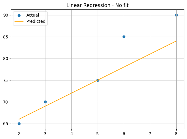

our initial line (prediction) we could say that it is not a good fit for the data, but here we are going to search for the best fit line using gradient descent.

import numpy as np


def loss_mse(y_true, predicted):
    return np.mean((y_true - predicted) ** 2)


initial_loss = loss_mse(y_true, no_fit_prediction)
print(f"Initial Loss: {initial_loss:.2f}")

Initial Loss: 17.40

Loss Function

We need to establish our loss metric. In this case, we are going to use the mean squared error (MSE) as our loss function.

The MSE formula is given by: \[ \text{MSE} = \frac{1}{n} \sum_{i=1}^{n} (y_i - \hat{y}_i)^2 \]

where:

• \(n\) is the number of observations,
• \(y_i\) is the true value,
• \(\hat{y}_i\) is the predicted value.

Manually calculating it

Point	\(x\)	\(y\)	calc	\(\hat{y}\)	\(y-\hat{y}\)	\((y-\hat{y})^2\)
a	\(2\)	\(65\)	\((3\times2) + 60\)	\(66\)	\(-1\)	\(1\)
b	\(3\)	\(70\)	\((3\times3) + 60\)	\(69\)	\(1\)	\(1\)
c	\(5\)	\(75\)	\((3\times5) + 60\)	\(75\)	\(0\)	\(0\)
d	\(6\)	\(85\)	\((3\times6) + 60\)	\(78\)	\(7\)	\(49\)
e	\(8\)	\(90\)	\((3\times8) + 60\)	\(84\)	\(6\)	\(36\)

then, \[MSE = \frac{1 + 1 + 0 + 49 + 36}{ 5} = 17.40\]

Gradient Descent: The Intuition

Now that we have a way to measure how “wrong” our line is (the MSE), we need a systematic way to make it “right.”

Imagine you are standing on a mountain in a thick fog. Your goal is to reach the lowest point in the valley, but you can’t see the path. What would you do? You would likely feel the slope of the ground with your feet and take a small step in the direction where the ground slopes downward.

In linear regression, our “mountain” is the Loss Surface. The altitude is our MSE, and our coordinates are the parameters \(m\) and \(b\). Gradient Descent is the process of calculating the slope (the gradient) at our current position and taking steps “downhill” to minimize the loss.

• Learning Rate: This is our “step size.” If it’s too large, we might overstep the valley. If it’s too small, it will take forever to reach the bottom.

The Math Behind the Gradients

To find the direction of the steepest descent, we use Partial Derivatives. We want to know how the MSE changes when we nudge \(m\) or \(b\).

Recall our MSE formula: \[\text{MSE} = \frac{1}{n} \sum_{i=1}^{n} (y_i - (mx_i + b))^2\]

Using the Chain Rule, we can derive the gradients for \(m\) and \(b\):

Gradient with respect to \(m\):

\[\frac{\partial \text{MSE}}{\partial m} = \frac{2}{n} \sum_{i=1}^{n} (y_i - \hat{y}_i) \cdot (-x_i) = - \frac{2}{n} \sum_{i=1}^{n} x_i(y_i - \hat{y}_i)\]

Gradient with respect to \(b\):

\[\frac{\partial \text{MSE}}{\partial b} = \frac{2}{n} \sum_{i=1}^{n} (y_i - \hat{y}_i) \cdot (-1) = - \frac{2}{n} \sum_{i=1}^{n} (y_i - \hat{y}_i)\]

In our code below, these are represented as dm and db. Notice how np.mean handles the \(\frac{1}{n} \sum\) part of the equation!

from plot_utils import plot_slope


def update(X, y_true, y_pred, m, b, learning_rate, plot=False):
    dm = -2 * np.mean(X * (y_true - y_pred))
    db = -2 * np.mean(y_true - y_pred)
    new_m = m - learning_rate * dm
    new_b = b - learning_rate * db
    if plot:
        print(f'{loss_mse(y_true, y_pred)}')
        print(f"new_m{new_m} - new_b{new_b} -> dm{dm} - db{db}")
        plot_slope(new_m, new_b)
    return new_m, new_b

m = 0.0
b = 0.0
epochs = 3000
learning_rate = 0.01
loss_history = []
slope_history = []

for epoch in range(epochs):
    y_pred = predict(X, m, b)
    current_loss = loss_mse(y_true, y_pred)
    loss_history.append(current_loss)

    # if epoch < 4:
    #     plot_fit(X, y_true, y_pred, title=f"Fit epoch {epoch + 1}", show_error=True)

    m, b = update(X, y_true, y_pred, m, b, learning_rate, plot=False)
    slope_history.append((m, b))

    if epoch == epochs - 1:
        final_loss = current_loss
        print(f"Final Loss: {final_loss:.4f}")
        print(f"Final Slope: {m:.4f}, Final Intercept: {b:.4f}")

Final Loss: 3.4649
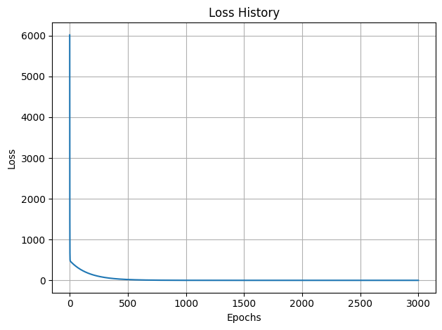
Final Slope: 4.2550, Final Intercept: 56.5754

Visualizing Convergence and Stagnation

We can plot the loss_history to see how the algorithm successfully minimized the error over time.

Notice that at the beginning, the loss drops drastically. This is because we are far from the optimal solution, and the gradients are large. However, as we approach the bottom of the valley, the improvements become marginal.

Passing a certain point (often called convergence), the model stops having good improvement, and further training yields insignificant gains. This is why we don’t need to train for an infinite number of epochs!

from plot_utils import plot_interactive_loss
plot_interactive_loss(loss_history)

The update function

This is how we find a better value for \(m\) and \(b\).

in simple terms, we identify the direction where we can improve, then we move to that direction at the rate of the learning_rate. as an example, we are going to manually calculate the first three iterations, and our starting point is \(m = 0\) and \(b = 0\)

flowchart TB
  A[Get the **predictions**<br>using predict] --> B(Calculate the Loss)
  B --> C{significant difference<br>with the previous loss?<br>or<br>still on the<br>epoch threshold?}
  C -- no --> D[We got our best *m*odel]
  C -- yes --> E((update <br>the weights))
  E -- "with the<br>updated<br>weights" --> A

First Epoch

The first epoch prediction is all \(0\).

Point	\(x\)	\(\hat{y}\)	\(y\)
a	2	0	65
b	3	0	70
c	5	0	75
d	6	0	85
e	8	0	90

\(X \times y_i - \hat{y}_i = [2,3,5,6,8] \times [65,70,75,85,90] = [130,210,375,510,720]\)

\(np.mean(X \times (y_i - \hat{y}_i)) = \frac{130+210+375+510+720}{5} = 389\)

\(np.mean(y_i - \hat{y}_i) = \frac{65+70+75+85+90}{5} = 77\)

\(dm = -2 \times 389 = -778\)

\(db = -2 \times 77 = -154\)

\(m_{new} = m - \text{learning rate} * dm = 0 - 0.01\times(-778) = 7.78\) \(b_{new} = b - \text{learning rate} * db = 0 - 0.01\times(-154) = 1.54\)

Calculating the Loss

\(\frac{65^2+70^2+75^2+85^2+90^2}{5} = 6015\)

Second and Third Epoch

For the following iterations, the steps remain identical, but our starting weights and predictions change as we learn.

NoteView Detailed Math for Epochs 2 & 3

Second Epoch

We use the updated \(m = 7.78\) and \(b = 1.54\)

\[\text{point } a \text{, our } \hat{y} = 7.78\times2 + 1.54 = 17.1\] \[\text{point } b \text{, our } \hat{y} = 7.78\times3 + 1.54 = 24.88\] \[\text{point } c \text{, our } \hat{y} = 7.78\times5 + 1.54 = 40.44\] \[\text{point } d \text{, our } \hat{y} = 7.78\times6 + 1.54 = 48.22\] \[\text{point } e \text{, our } \hat{y} = 7.78\times8 + 1.54 = 63.78\]

Point	\(x\)	\(\hat{y}\)	\(y\)	\(y-\hat{y}\)
a	2	17.1	65	47.9
b	3	24.88	70	45.12
c	5	40.44	75	34.56
d	6	48.22	85	36.78
e	8	63.78	90	26.22

\(X \times y_i - \hat{y}_i = [2,3,5,6,8] \times [47.9,45.12,34.56,36.78,26.22] = [95.8,135.36,172.8,220.68, 209.76]\)

\(np.mean(X \times (y_i - \hat{y}_i)) = \frac{95.8+135.36+172.8+220.68+ 209.76 }{5} = 166.88\)

\(np.mean(y_i - \hat{y}_i) = \frac{47.9+45.12+34.56+36.78+26.22}{5} = 38.116\)

\(dm = -2 \times 166.88 = -333.76\)

\(db = -2 \times 38.116 = -76.23\)

\(m_{new} = m - \text{learning rate} * dm = 7.78 - 0.01\times(-333.76) = 11.11\)

\(b_{new} = b - \text{learning rate} * db = 1.54 - 0.01\times(-76.23) = 2.30\)

Calculating the Loss

\(\frac{47.9^2+45.12^2+34.56^2+36.78^2+26.22^2}{5} = 1512.97\)

so the difference between the first loss and this one is \[6015 \rightarrow 1512.97\]

Third Epoch

from the previous iteration we have \(m = 11.11\) and \(b = 2.30\)

\[\text{point } a \text{, our } \hat{y} = 11.11\times2 + 2.30 = 24.53\] \[\text{point } b \text{, our } \hat{y} = 11.11\times3 + 2.30 = 35.65\] \[\text{point } c \text{, our } \hat{y} = 11.11\times5 + 2.30 = 57.89\] \[\text{point } d \text{, our } \hat{y} = 11.11\times6 + 2.30 = 69.00\] \[\text{point } e \text{, our } \hat{y} = 11.11\times8 + 2.30 = 91.24\]

Point	\(x\)	\(\hat{y}\)	\(y\)	\(y-\hat{y}\)
a	2	24.53	65	40.46
b	3	35.65	70	34.34
c	5	57.89	75	17.11
d	6	69.00	85	15.99
e	8	91.24	90	-1.24

\(X \times y_i - \hat{y}_i = [2,3,5,6,8] \times [40.46, 34.34, 17.11, 15.99, -1.24] = [80.92, 103.03, 85.54, 95.95, -9.94]\)

\(np.mean(X \times (y_i - \hat{y}_i)) = \frac{80.92+ 103.03+ 85.54+ 95.95 -9.94}{5} = 71.1\)

\(np.mean(y_i - \hat{y}_i) = \frac{40.46+ 34.34+ 17.11+ 15.99+ -1.24}{5} = 21.33\)

\(dm = -2 \times 71.1 = -142.20\)

\(db = -2 \times 21.33 = -42.66\)

\(m_{new} = m - \text{learning rate} * dm = 11.11 - 0.01\times(-142.20) = 12.53\)

\(b_{new} = b - \text{learning rate} * db = 2.30 - 0.01\times(-42.66) = 2.72\)

Calculating the Loss

\(\frac{80.92^2+ 103.03^2+ 85.54^2+ 95.95^2 + (- 9.94)^2}{5} = 673.36\)

for this epoch we went lower than the half of the previous epoch \[1512.97 \rightarrow 673.36\]

As we continue, the steps become smaller as we approach the bottom of the “valley.”

Note Theoretically at some point we are going to stop having this improvement on the loss function, and when that happens, it is wise to stop the iterations.

Here is an interactive plot, where we plot the predicted line across epoch, so we can check the evolution and stagnation of the learning.

from plot_utils import plot_loss, create_interactive_line_chart

create_interactive_line_chart(dataset=slope_history,
                              scatter_x=X,
                              scatter_y=y_true,
                              x_range=(0, 8))

fit_predicted = predict(X, m, b)
plot_fit(X, y_true, fit_predicted, "Linear Regression - Fit")

fit_loss = loss_mse(y_true, fit_predicted)
plot_loss(loss_history)
print(f"Fit (final) Loss: {fit_loss:.2f}")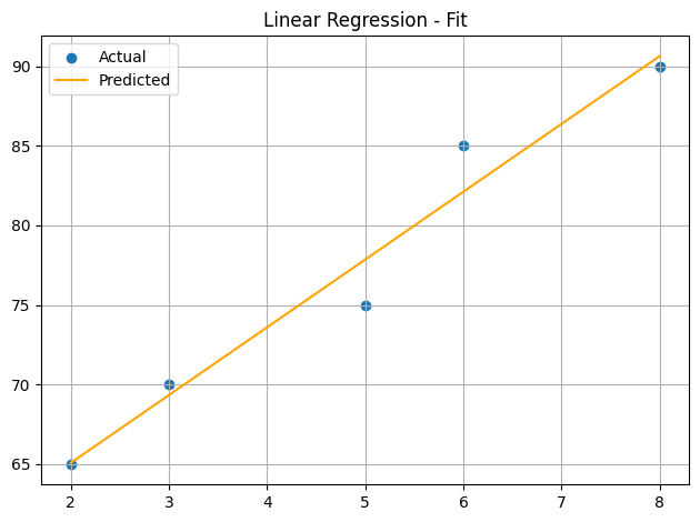

Fit (final) Loss: 3.46

Takeaways

• Linear Regression is about finding the line that best represents the trend in your data by minimizing a loss function (like MSE).
• The Gradients (derived using Calculus) tell us exactly how much and in what direction to nudge our parameters \(m\) and \(b\) to reduce the error.
• Gradient Descent iteratively applies these nudges until the loss stabilizes, signifying we’ve reached the bottom of the “valley.”
• Automation: While we used a fixed number of epochs, real-world implementations often use “early stopping” or convergence thresholds to stop training automatically.