Predicting Car Insurance Claims

Only about 6% of the policies in this dataset ever file a claim. That imbalance makes claim prediction a genuinely hard problem: accuracy is meaningless, and a model that never flags anyone scores 94%. This notebook walks the full pipeline — data engineering, multicollinearity pruning, statistical feature selection, a model bake-off, and business-aware threshold tuning — with the goal of catching as many real claims as possible at an acceptable false-alarm rate.

Code

import pandas as pd

df_claim = pd.read_csv('data/train.csv')

Insurance Data

Variable	Description
policy_id	Unique identifier of the policyholder
policy_tenure	Time period of the policy
age_of_car	Normalized age of the car in years
age_of_policyholder	Normalized age of policyholder in years
area_cluster	Area cluster of the policyholder
population	density Population density of the city (Policyholder City)
make	Encoded Manufacturer/company of the car
segment	Segment of the car (A/ B1/ B2/ C1/ C2)
model	Encoded name of the car
fuel_type	Type of fuel used by the car
max_torque	Maximum Torque generated by the car (Nm@rpm)
max_power	Maximum Power generated by the car (bhp@rpm)
engine_type	Type of engine used in the car
airbags	Number of airbags installed in the car
is_esc	Boolean flag indicating whether Electronic Stability Control (ESC) is present in the car or not.
is_adjustable_steering	Boolean flag indicating whether the steering wheel of the car is adjustable or not.
is_tpms	Boolean flag indicating whether Tyre Pressure Monitoring System (TPMS) is present in the car or not.
is_parking_sensors	Boolean flag indicating whether parking sensors are present in the car or not.
is_parking_camera	Boolean flag indicating whether the parking camera is present in the car or not.
rear_brakes_type	Type of brakes used in the rear of the car
displacement	Engine displacement of the car (cc)
cylinder	Number of cylinders present in the engine of the car
transmission_type	Transmission type of the car
gear_box	Number of gears in the car
steering_type	Type of the power steering present in the car
turning_radius	The space a vehicle needs to make a certain turn (Meters)
length	Length of the car (Millimetre)
width	Width of the car (Millimetre)
height	Height of the car (Millimetre)
gross_weight	The maximum allowable weight of the fully-loaded car, including passengers, cargo and equipment (Kg)
is_front_fog_lights	Boolean flag indicating whether front fog lights are available in the car or not.
is_rear_window_wiper	Boolean flag indicating whether the rear window wiper is available in the car or not.
is_rear_window_washer	Boolean flag indicating whether the rear window washer is available in the car or not.
is_rear_window_defogger	Boolean flag indicating whether rear window defogger is available in the car or not.
is_brake_assist	Boolean flag indicating whether the brake assistance feature is available in the car or not.
is_power_door_lock	Boolean flag indicating whether a power door lock is available in the car or not.
is_central_locking	Boolean flag indicating whether the central locking feature is available in the car or not.
is_power_steering	Boolean flag indicating whether power steering is available in the car or not.
is_driver_seat_height_adjustable	Boolean flag indicating whether the height of the driver seat is adjustable or not.
is_day_night_rear_view_mirror	Boolean flag indicating whether day & night rearview mirror is present in the car or not.
is_ecw	Boolean flag indicating whether Engine Check Warning (ECW) is available in the car or not.
is_speed_alert	Boolean flag indicating whether the speed alert system is available in the car or not.
ncap_rating	Safety rating given by NCAP (out of 5)
is_claim	Outcome: Boolean flag indicating whether the policyholder file a claim in the next 6 months or not.

Code

print(df_claim.head())
df_claim.info()

  policy_id  policy_tenure  age_of_car  age_of_policyholder area_cluster  \
0   ID00001       0.515874        0.05             0.644231           C1   
1   ID00002       0.672619        0.02             0.375000           C2   
2   ID00003       0.841110        0.02             0.384615           C3   
3   ID00004       0.900277        0.11             0.432692           C4   
4   ID00005       0.596403        0.11             0.634615           C5   

   population_density  make segment model fuel_type  ... is_brake_assist  \
0                4990     1       A    M1       CNG  ...              No   
1               27003     1       A    M1       CNG  ...              No   
2                4076     1       A    M1       CNG  ...              No   
3               21622     1      C1    M2    Petrol  ...             Yes   
4               34738     2       A    M3    Petrol  ...              No   

  is_power_door_locks is_central_locking  is_power_steering  \
0                  No                 No                Yes   
1                  No                 No                Yes   
2                  No                 No                Yes   
3                 Yes                Yes                Yes   
4                 Yes                Yes                Yes   

  is_driver_seat_height_adjustable is_day_night_rear_view_mirror is_ecw  \
0                               No                            No     No   
1                               No                            No     No   
2                               No                            No     No   
3                              Yes                           Yes    Yes   
4                               No                           Yes    Yes   

  is_speed_alert ncap_rating is_claim  
0            Yes           0        0  
1            Yes           0        0  
2            Yes           0        0  
3            Yes           2        0  
4            Yes           2        0  

[5 rows x 44 columns]
<class 'pandas.DataFrame'>
RangeIndex: 58592 entries, 0 to 58591
Data columns (total 44 columns):
 #   Column                            Non-Null Count  Dtype  
---  ------                            --------------  -----  
 0   policy_id                         58592 non-null  str    
 1   policy_tenure                     58592 non-null  float64
 2   age_of_car                        58592 non-null  float64
 3   age_of_policyholder               58592 non-null  float64
 4   area_cluster                      58592 non-null  str    
 5   population_density                58592 non-null  int64  
 6   make                              58592 non-null  int64  
 7   segment                           58592 non-null  str    
 8   model                             58592 non-null  str    
 9   fuel_type                         58592 non-null  str    
 10  max_torque                        58592 non-null  str    
 11  max_power                         58592 non-null  str    
 12  engine_type                       58592 non-null  str    
 13  airbags                           58592 non-null  int64  
 14  is_esc                            58592 non-null  str    
 15  is_adjustable_steering            58592 non-null  str    
 16  is_tpms                           58592 non-null  str    
 17  is_parking_sensors                58592 non-null  str    
 18  is_parking_camera                 58592 non-null  str    
 19  rear_brakes_type                  58592 non-null  str    
 20  displacement                      58592 non-null  int64  
 21  cylinder                          58592 non-null  int64  
 22  transmission_type                 58592 non-null  str    
 23  gear_box                          58592 non-null  int64  
 24  steering_type                     58592 non-null  str    
 25  turning_radius                    58592 non-null  float64
 26  length                            58592 non-null  int64  
 27  width                             58592 non-null  int64  
 28  height                            58592 non-null  int64  
 29  gross_weight                      58592 non-null  int64  
 30  is_front_fog_lights               58592 non-null  str    
 31  is_rear_window_wiper              58592 non-null  str    
 32  is_rear_window_washer             58592 non-null  str    
 33  is_rear_window_defogger           58592 non-null  str    
 34  is_brake_assist                   58592 non-null  str    
 35  is_power_door_locks               58592 non-null  str    
 36  is_central_locking                58592 non-null  str    
 37  is_power_steering                 58592 non-null  str    
 38  is_driver_seat_height_adjustable  58592 non-null  str    
 39  is_day_night_rear_view_mirror     58592 non-null  str    
 40  is_ecw                            58592 non-null  str    
 41  is_speed_alert                    58592 non-null  str    
 42  ncap_rating                       58592 non-null  int64  
 43  is_claim                          58592 non-null  int64  
dtypes: float64(4), int64(12), str(28)
memory usage: 19.7 MB

1. Data Audit

Some variable types don’t make sense at first glance, so we audit them before modeling.

policy_id should be dropped for the feature selection.

Code

import matplotlib.pyplot as plt
import pandas as pd
import seaborn as sns

unique_counts = {}
for col in df_claim.columns:
    if (df_claim[col].dtype == 'object' or df_claim[col].dtype == 'str') and col != 'policy_id':
        unique_counts[col] = df_claim[col].nunique()

df_unique = pd.DataFrame(list(unique_counts.items()), columns=['Feature', 'Unique_Count'])
df_unique = df_unique.sort_values(by='Unique_Count', ascending=False)

plt.figure(figsize=(12, 10))

sns.barplot(
    x='Unique_Count',
    y='Feature',
    data=df_unique,
    palette='viridis',
    hue='Feature',
    legend=False
)

plt.title('Number of Unique Values per Categorical Feature', fontsize=16, pad=15)
plt.xlabel('Number of Unique Categories', fontsize=12)
plt.ylabel('Feature Name', fontsize=12)

for index, value in enumerate(df_unique['Unique_Count']):
    plt.text(value + 0.2, index, str(value), va='center', fontsize=10)

plt.tight_layout()
plt.show()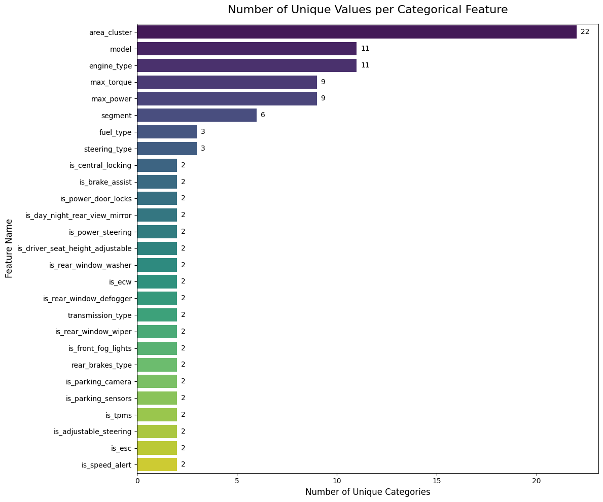

Code

print("Possible model:")
print(pd.Categorical(df_claim['model']).unique().tolist())
print("Possible segments:")
print(pd.Categorical(df_claim['segment']).unique().tolist())
print("Possible engine types:")
print(pd.Categorical(df_claim['engine_type']).unique().tolist())

Possible model:
['M1', 'M2', 'M3', 'M4', 'M5', 'M6', 'M7', 'M8', 'M9', 'M10', 'M11']
Possible segments:
['A', 'C1', 'C2', 'B2', 'B1', 'Utility']
Possible engine types:
['F8D Petrol Engine', '1.2 L K12N Dualjet', '1.0 SCe', '1.5 L U2 CRDi', '1.5 Turbocharged Revotorq', 'K Series Dual jet', '1.2 L K Series Engine', 'K10C', 'i-DTEC', 'G12B', '1.5 Turbocharged Revotron']

2. Data Engineering

Several categorical columns contain high-cardinality values; naive dummy encoding would dramatically expand the feature space.
Many vehicle specifications are structurally redundant (for example, the specific combination of car model, segment, and engine type uniquely determines many of the boolean feature flags).

The Plan

To preserve signal while preventing high-cardinality explosion, any category that accounts for less than 1% of observations (min_frequency=0.01) is bucketed: - If two or more categories are rare within a column, they are grouped into a consolidated 'Other' category. - If only a single category is rare, it is absorbed into the majority class.

By bucketing rare categories, we protect downstream models from overfitting to sparse values that lack sufficient sample support for generalization.

Code

def clean_insurance_data(df, min_frequency=0.01):
    """
    Cleans the specific car insurance dataset for statsmodels regression.
    Handles string parsing, binary mapping, rare category bucketing, and dummy encoding.
    Any category with fewer `min_frequency` (total rows are 58,592 so 586 as default value)
    """
    print("Starting data clean-up...")
    df_clean = df.copy()

    if 'policy_id' in df_clean.columns:
        df_clean = df_clean.drop('policy_id', axis=1)
        print("Dropped 'policy_id'.")

    print("Parsing torque and power strings into numbers...")
    regex_pattern = r'([\d\.]+).*?@.*?([\d\.]+)'

    if 'max_torque' in df_clean.columns:
        df_clean[['torque_value', 'torque_rpm']] = df_clean['max_torque'].str.extract(regex_pattern).astype(float)
        df_clean = df_clean.drop('max_torque', axis=1)

    if 'max_power' in df_clean.columns:
        df_clean[['power_value', 'power_rpm']] = df_clean['max_power'].str.extract(regex_pattern).astype(float)
        df_clean = df_clean.drop('max_power', axis=1)

    print("Mapping 'is_' columns to 1 and 0...")
    binary_cols = [col for col in df_clean.columns if col.startswith('is_') and col != 'is_claim']

    for col in binary_cols:
        if df_clean[col].dtype == 'object':
            df_clean[col] = df_clean[col].map({'Yes': 1, 'No': 0, 'yes': 1, 'no': 0})

    df_clean = df_clean.dropna()

    print(f"Bucketing rare categories (threshold: < {min_frequency * 100}% of data)...")
    categorical_cols = df_clean.select_dtypes(include=['object', 'str']).columns

    for col in categorical_cols:
        frequencies = df_clean[col].value_counts(normalize=True)
        rare_categories = frequencies[frequencies < min_frequency].index

        if len(rare_categories) > 1:
            df_clean[col] = df_clean[col].replace(rare_categories, 'Other')
            print(f"  - '{col}': grouped {len(rare_categories)} rare values into 'Other'")

        elif len(rare_categories) == 1:
            majority_class = frequencies.idxmax()
            df_clean[col] = df_clean[col].replace(rare_categories, majority_class)
            print(f"  - '{col}': absorbed 1 sparse value into majority class '{majority_class}'")

    print("Applying dummy encoding (drop_first=True)...")
    df_clean = pd.get_dummies(df_clean, drop_first=True, dtype=float)

    print("-" * 40)
    print(f"Clean-up complete! Final dataset shape: {df_clean.shape}")

    X = df_clean.drop('is_claim', axis=1)
    y = df_clean['is_claim']

    return X, y

Code

import matplotlib.pyplot as plt
import seaborn as sns
import numpy as np


def plot_correlation_heatmap(df_features, title):
    """
    Plots a highly formatted, readable correlation heatmap for large datasets.
    """
    corr = df_features.corr()
    mask = np.triu(np.ones_like(corr, dtype=bool))
    plt.figure(figsize=(20, 16))

    sns.heatmap(
        corr,
        mask=mask,
        cmap='coolwarm',
        vmin=-1, vmax=1,
        square=True,
        linewidths=.5,
        cbar_kws={"shrink": .5}
    )

    plt.title(title, fontsize=20, pad=20)
    plt.tight_layout()
    plt.show()

Code

X, y = clean_insurance_data(df_claim)
plot_correlation_heatmap(X, "Correlation Heatmap BEFORE VIF (High Multicollinearity)")

Starting data clean-up...
Dropped 'policy_id'.
Parsing torque and power strings into numbers...
Mapping 'is_' columns to 1 and 0...
Bucketing rare categories (threshold: < 1.0% of data)...
  - 'area_cluster': grouped 6 rare values into 'Other'
  - 'model': absorbed 1 sparse value into majority class 'M1'
  - 'engine_type': absorbed 1 sparse value into majority class 'F8D Petrol Engine'
  - 'is_speed_alert': absorbed 1 sparse value into majority class 'Yes'
Applying dummy encoding (drop_first=True)...
----------------------------------------
Clean-up complete! Final dataset shape: (58592, 81)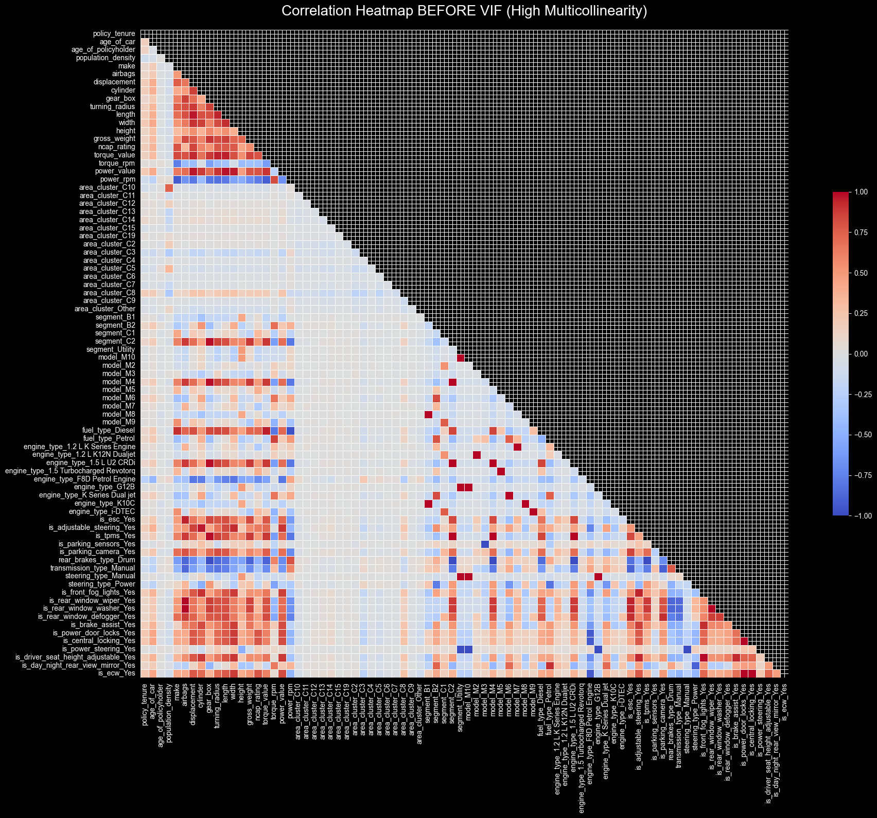

3. Multicollinearity and VIF

Multicollinearity occurs when two or more predictor variables in a regression model are highly linearly correlated, providing overlapping information about the outcome.

For example, in real estate pricing, square footage and room count—or redundant location proxies like zip code, county, and neighborhood—provide heavily overlapping signals.

Why is it harmful?

Collinearity inflates the variance of coefficient estimates and destabilizes parameter signs. In a linear model, the solver may compensate by assigning an artificially large positive weight to one collinear feature and a large negative weight to its duplicate. When evaluating unseen data where that balance shifts slightly, predictions can swing wildly, destroying interpretability and generalizability.

graph LR
A( Model gets confused ) --> B( Math breaks down ) --> C( You can't trust the numbers) --> D( You can't interpret the results ) --> E( You can't act on them )

Code

from statsmodels_utils import calculate_and_drop_vif

X_clean, dropped_features = calculate_and_drop_vif(X)

Starting VIF Multicollinearity Check...

----------------------------------------
Dropped: 'make' (VIF: inf)
Dropped: 'airbags' (VIF: inf)
Dropped: 'displacement' (VIF: inf)
Dropped: 'cylinder' (VIF: inf)
Dropped: 'gear_box' (VIF: inf)
Dropped: 'turning_radius' (VIF: inf)
Dropped: 'length' (VIF: inf)
Dropped: 'width' (VIF: inf)
Dropped: 'height' (VIF: inf)
Dropped: 'gross_weight' (VIF: inf)
Dropped: 'ncap_rating' (VIF: inf)
Dropped: 'torque_value' (VIF: inf)
Dropped: 'torque_rpm' (VIF: inf)
Dropped: 'power_value' (VIF: inf)
Dropped: 'power_rpm' (VIF: inf)
Dropped: 'segment_B1' (VIF: inf)
Dropped: 'segment_B2' (VIF: inf)
Dropped: 'segment_C1' (VIF: inf)
Dropped: 'segment_C2' (VIF: inf)
Dropped: 'segment_Utility' (VIF: inf)
Dropped: 'model_M10' (VIF: inf)
Dropped: 'model_M2' (VIF: inf)
Dropped: 'model_M3' (VIF: inf)
Dropped: 'model_M4' (VIF: inf)
Dropped: 'model_M5' (VIF: inf)
Dropped: 'model_M6' (VIF: inf)
Dropped: 'model_M7' (VIF: inf)
Dropped: 'model_M8' (VIF: inf)
Dropped: 'model_M9' (VIF: inf)
Dropped: 'fuel_type_Diesel' (VIF: inf)
Dropped: 'fuel_type_Petrol' (VIF: inf)
Dropped: 'engine_type_1.2 L K Series Engine' (VIF: inf)
Dropped: 'engine_type_1.2 L K12N Dualjet' (VIF: inf)
Dropped: 'engine_type_1.5 L U2 CRDi' (VIF: inf)
Dropped: 'engine_type_1.5 Turbocharged Revotorq' (VIF: inf)
Dropped: 'engine_type_F8D Petrol Engine' (VIF: inf)
Dropped: 'engine_type_G12B' (VIF: inf)
Dropped: 'engine_type_K Series Dual jet' (VIF: inf)
Dropped: 'engine_type_K10C' (VIF: inf)
Dropped: 'engine_type_i-DTEC' (VIF: inf)
Dropped: 'is_esc_Yes' (VIF: inf)
Dropped: 'is_adjustable_steering_Yes' (VIF: inf)
Dropped: 'is_tpms_Yes' (VIF: inf)
Dropped: 'is_parking_sensors_Yes' (VIF: inf)
Dropped: 'is_parking_camera_Yes' (VIF: inf)
Dropped: 'rear_brakes_type_Drum' (VIF: inf)
Dropped: 'steering_type_Manual' (VIF: inf)
Dropped: 'is_rear_window_wiper_Yes' (VIF: inf)
Dropped: 'is_power_door_locks_Yes' (VIF: inf)
Dropped: 'is_central_locking_Yes' (VIF: inf)
Dropped: 'is_driver_seat_height_adjustable_Yes' (VIF: 178.12)
Dropped: 'is_front_fog_lights_Yes' (VIF: 18.56)
Dropped: 'population_density' (VIF: 17.91)
Dropped: 'is_rear_window_washer_Yes' (VIF: 12.83)
Dropped: 'steering_type_Power' (VIF: 11.69)
Dropped: 'area_cluster_C8' (VIF: 8.20)
----------------------------------------
VIF Check Complete!
Features dropped: 56

Code

print(dropped_features)

['make', 'airbags', 'displacement', 'cylinder', 'gear_box', 'turning_radius', 'length', 'width', 'height', 'gross_weight', 'ncap_rating', 'torque_value', 'torque_rpm', 'power_value', 'power_rpm', 'segment_B1', 'segment_B2', 'segment_C1', 'segment_C2', 'segment_Utility', 'model_M10', 'model_M2', 'model_M3', 'model_M4', 'model_M5', 'model_M6', 'model_M7', 'model_M8', 'model_M9', 'fuel_type_Diesel', 'fuel_type_Petrol', 'engine_type_1.2 L K Series Engine', 'engine_type_1.2 L K12N Dualjet', 'engine_type_1.5 L U2 CRDi', 'engine_type_1.5 Turbocharged Revotorq', 'engine_type_F8D Petrol Engine', 'engine_type_G12B', 'engine_type_K Series Dual jet', 'engine_type_K10C', 'engine_type_i-DTEC', 'is_esc_Yes', 'is_adjustable_steering_Yes', 'is_tpms_Yes', 'is_parking_sensors_Yes', 'is_parking_camera_Yes', 'rear_brakes_type_Drum', 'steering_type_Manual', 'is_rear_window_wiper_Yes', 'is_power_door_locks_Yes', 'is_central_locking_Yes', 'is_driver_seat_height_adjustable_Yes', 'is_front_fog_lights_Yes', 'population_density', 'is_rear_window_washer_Yes', 'steering_type_Power', 'area_cluster_C8']

53018VIF_i = rac{1}{1 - R_i^2}53018

Interpreting VIF Scores & Selecting the Threshold

= 1.0$ (^2 = 0%$): Completely orthogonal; zero correlation with other features.
= 5.0$ (^2 = 80%$): Our cutoff threshold. A standard statistical rule of thumb in econometrics and regression modeling. A VIF $> 5.0$ indicates that more than %$ of that variable’s variance is already captured by other predictors in the dataset.
**= $ (^2 = 100%$):** Perfect linear dependency. The auxiliary regression fits with ^2 = 1.0$, resulting in division by zero. In our dataset, this occurs when vehicle specs (e.g., engine type, cylinders, brake systems) are completely deterministic given the car model.

The Iterative Pruning Rule

We apply a strict stopping rule of $\le 5.0$: 1. Calculate VIF across all current features in the dataset. 2. Identify the single feature with the highest VIF exceeding .0$ and drop it. 3. Recalculate VIF across all remaining features (dropping one collinear variable immediately deflates the inflated VIF scores of its correlated peers). 4. Repeat iteratively until every remaining feature satisfies $\le 5.0$.

Code

plot_correlation_heatmap(X_clean, "Correlation Heatmap AFTER VIF (Independent Multicollinearity)")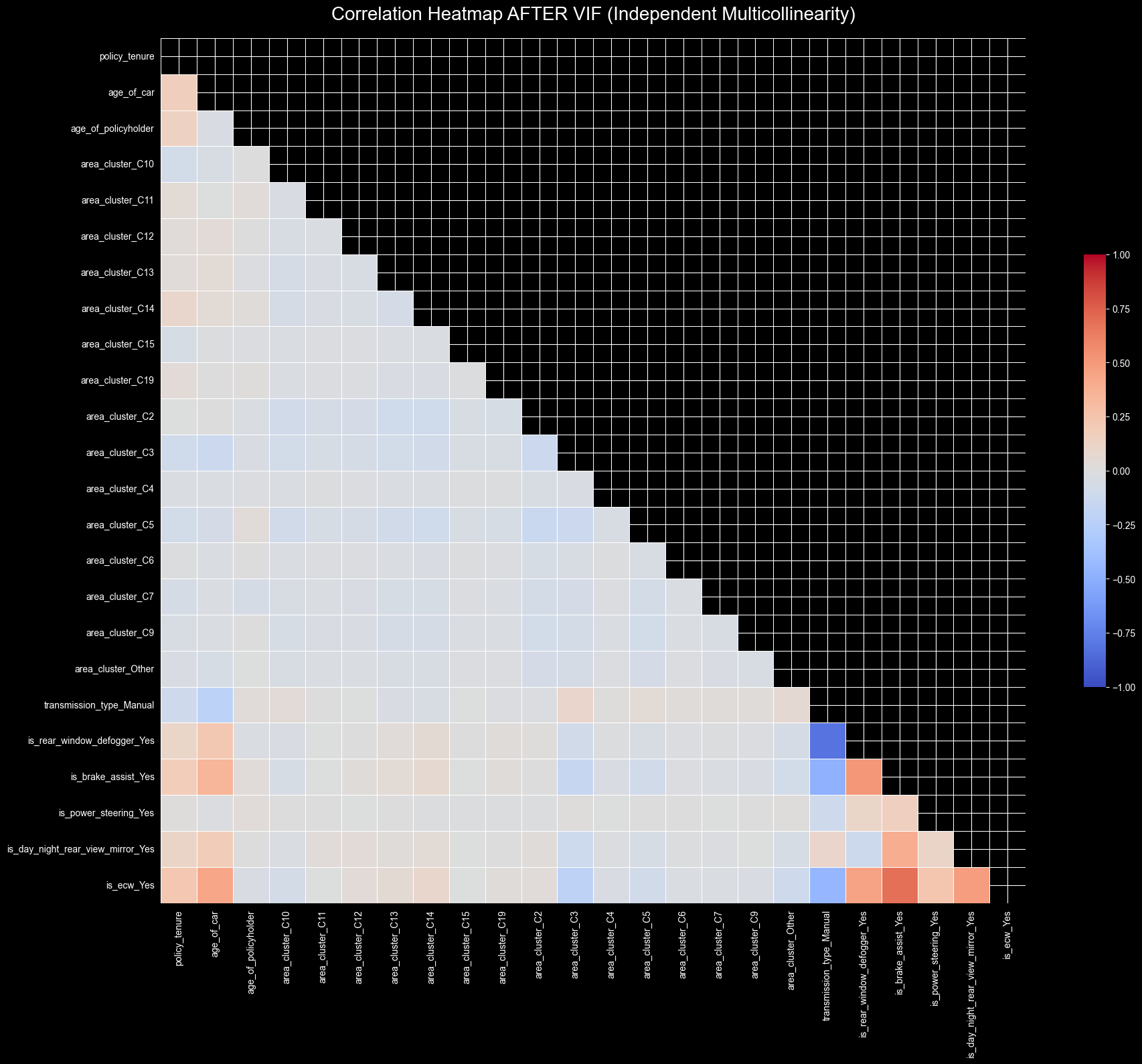

4. Statistical Modeling: Stepwise Logistic Regression

Before deploying complex machine learning algorithms, we fit an interpretable statistical baseline using Bidirectional Stepwise Logistic Regression (stepwise_selection_logit).

How Stepwise Selection Works

Starting with an empty model, the algorithm tests features in alternating steps:

Adding features (Forward Step): It tests every feature outside the model and adds the single one with the strongest statistical evidence ($p < 0.05$).
Removing features (Backward Step): After adding a new feature, it checks if any previously added feature became redundant. If an older feature’s $p$-value rose above $0.05$, it gets dropped.
When does it stop? The loop finishes when the model stabilizes:
- Nothing left outside is strong enough to enter (no feature has $p < 0.05$).
- Nothing inside is weak enough to leave (all features stay $p \le 0.05$).

Why This Matters for Insurance

This distills the post-VIF feature space down to the core subset with rigorous statistical evidence of predicting claims. The resulting log-odds coefficients ($\beta$) provide underwriters with transparent, auditable factors rather than a black-box model.

Code

from statsmodels_utils import stepwise_selection_logit

print(X_clean.columns.tolist())
best_model, final_features = stepwise_selection_logit(X_clean, y, threshold_in=0.05, threshold_out=0.05)

['policy_tenure', 'age_of_car', 'age_of_policyholder', 'area_cluster_C10', 'area_cluster_C11', 'area_cluster_C12', 'area_cluster_C13', 'area_cluster_C14', 'area_cluster_C15', 'area_cluster_C19', 'area_cluster_C2', 'area_cluster_C3', 'area_cluster_C4', 'area_cluster_C5', 'area_cluster_C6', 'area_cluster_C7', 'area_cluster_C9', 'area_cluster_Other', 'transmission_type_Manual', 'is_rear_window_defogger_Yes', 'is_brake_assist_Yes', 'is_power_steering_Yes', 'is_day_night_rear_view_mirror_Yes', 'is_ecw_Yes']
Starting Stepwise Selection using Logit...

----------------------------------------
Added:   'policy_tenure' (p-value: 0.0000)
Added:   'age_of_car' (p-value: 0.0000)
Added:   'area_cluster_C3' (p-value: 0.0015)
Added:   'area_cluster_C2' (p-value: 0.0022)
Added:   'is_brake_assist_Yes' (p-value: 0.0062)
Added:   'area_cluster_C14' (p-value: 0.0269)
Added:   'age_of_policyholder' (p-value: 0.0283)
Added:   'area_cluster_C4' (p-value: 0.0257)
Added:   'area_cluster_C10' (p-value: 0.0481)
Added:   'area_cluster_C9' (p-value: 0.0447)
Dropped: 'area_cluster_C14' (p-value: 0.0506)
----------------------------------------
Stepwise Selection Complete!
Final number of features: 9

Code

best_model.summary()

Logit Regression Results
Dep. Variable:	is_claim	No. Observations:	58592
Model:	Logit	Df Residuals:	58582
Method:	MLE	Df Model:	9
Date:	Wed, 16 Sep 2026	Pseudo R-squ.:	0.01877
Time:	20:29:12	Log-Likelihood:	-13669.
converged:	True	LL-Null:	-13930.
Covariance Type:	nonrobust	LLR p-value:	7.379e-107

	coef	std err	z	P>\|z\|	[0.025	0.975]
const	-3.2405	0.076	-42.579	0.000	-3.390	-3.091
policy_tenure	0.8462	0.044	19.136	0.000	0.760	0.933
age_of_car	-3.5342	0.349	-10.115	0.000	-4.219	-2.849
area_cluster_C3	0.1949	0.056	3.500	0.000	0.086	0.304
area_cluster_C2	0.1405	0.050	2.790	0.005	0.042	0.239
is_brake_assist_Yes	0.0946	0.037	2.535	0.011	0.021	0.168
age_of_policyholder	0.3080	0.136	2.258	0.024	0.041	0.575
area_cluster_C4	0.2916	0.148	1.968	0.049	0.001	0.582
area_cluster_C10	-0.1989	0.088	-2.271	0.023	-0.371	-0.027
area_cluster_C9	-0.1963	0.091	-2.158	0.031	-0.375	-0.018

Code

from statsmodels_utils import plot_coef

plot_coef(best_model)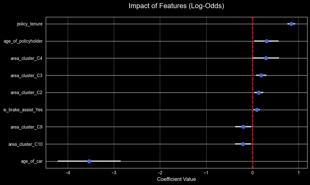

Key Insights from Feature Impacts (Log-Odds)

The regression table above and coefficient plot below display the estimated log-odds coefficients ($\beta$) with 95% confidence intervals from the Stepwise Logistic Regression model. The baseline (dashed line at $0.0$) represents no effect. Because coefficients represent log-odds, their exponentiated values yield the Odds Ratio ($OR = e^\beta$):

1. Vehicle Age is the Strongest Protective Factor (`age_of_car`: $\beta = -3.53$, $OR \approx 0.03$)

The Finding: Has the single largest effect size in the entire model. As vehicle age increases, claim probability plummets.
Insurance Rationale: Brand-new cars carry full comprehensive and collision coverage, and owners file claims for even minor cosmetic damage to protect vehicle resale value. For older cars, drivers often switch to liability-only coverage or absorb minor repair costs out-of-pocket because damage values fall below the deductible.

2. Policy Tenure Increases Claim Frequency (`policy_tenure`: $\beta = +0.85$, $OR \approx 2.33$)

The Finding: Longer policy relationships are strongly associated with higher claim probability ($>2\times$ odds increase per unit of normalized tenure).
Insurance Rationale: Brand-new policyholders exhibit lower claim frequency during initial onboarding periods, whereas long-tenured customers are more comfortable actively utilizing their coverage and navigating the claim process without fear of immediate policy cancellation.

3. Driver Demographics (`age_of_policyholder`: $\beta = +0.31$, $OR \approx 1.36$)

The Finding: Older policyholders exhibit a statistically significant $+36\%$ increase in the odds of filing a claim.
Insurance Rationale: Aligns with standard actuarial loss curves where older demographics show increased accident frequencies due to reduced night vision, slower reaction times, or higher medical severity in crashes.

4. Geographic Territory Segmentation (`area_cluster`)

High-Risk Territories: Clusters C4 ($\beta = +0.29$), C3 ($\beta = +0.19$), and C2 ($\beta = +0.14$) significantly elevate claim odds.
Low-Risk Territories: Clusters C9 ($\beta = -0.20$) and C10 ($\beta = -0.20$) significantly reduce claim odds.
Insurance Rationale: Demonstrates clear territorial risk segmentation driven by urban traffic congestion, road infrastructure quality, and regional claim fraud rates. Insurers can directly translate these into territorial rating factors (e.g., $+15\%$ to $+33\%$ surcharges for C2–C4 vs. $\approx 18\%$ discounts for C9–C10).

5. Safety Tech / Luxury Proxy (`is_brake_assist_Yes`: $\beta = +0.09$, $OR \approx 1.10$)

The Finding: Vehicles equipped with brake assistance show a slight $+10\%$ increase in claim odds.
Insurance Rationale: While safety tech prevents collisions, it serves as a proxy for newer, higher-trim vehicles equipped with costly sensors, cameras, and radar units in bumpers. Minor fender-benders that would cost $300 to fix on basic cars easily exceed the $1,000 deductible on tech-heavy vehicles, turning minor incidents into reported insurance claims.

5. Model Bake-Off

We now benchmark three model families under standardized conditions with 5-fold cross-validation and class_weight='balanced': - Logistic Regression (linear baseline, wrapped in a pipeline with StandardScaler to prevent CV fold leakage) - Random Forest (bagging ensemble, trained on unscaled features) - HistGradientBoosting (gradient boosting ensemble, trained on unscaled features)

Note on feature space: While Stepwise Selection in Section 4 isolated the key linear drivers for inference, we supply the full post-VIF feature space (X_clean) to the bake-off. This allows the non-linear ensembles to evaluate multi-way feature interactions that a linear logit model cannot represent.

Code

from sklearn.pipeline import Pipeline
from sklearn.preprocessing import StandardScaler
from sklearn.ensemble import HistGradientBoostingClassifier, RandomForestClassifier
from sklearn.linear_model import LogisticRegression
from sklearn.model_selection import GridSearchCV, train_test_split
import time

seed = 42

logReg = 'Logistic Regression'
forest = 'Random Forest'
hist = 'HistGradientBoosting'

models = {
    logReg: Pipeline([
        ('scaler', StandardScaler()),
        ('clf', LogisticRegression(class_weight='balanced', max_iter=1000, random_state=seed))
    ]),
    forest: RandomForestClassifier(class_weight='balanced', random_state=seed),
    hist: HistGradientBoostingClassifier(class_weight='balanced', random_state=seed)
}

param_grids = {
    logReg: {
        'clf__C': [0.01, 0.1, 1.0, 10.0],
        'clf__solver': ['liblinear', 'saga']
    },
    forest: {
        'n_estimators': [100, 300],
        'max_depth': [5, 10, 15],
        'min_samples_leaf': [2, 5, 10]
    },
    hist: {
        'learning_rate': [0.01, 0.05, 0.1],
        'max_iter': [100, 300],
        'max_depth': [3, 5, 7],
        'l2_regularization': [0.0, 1.0]
    }
}

best_models = {}
best_scores = {}

if 'const' in X_clean.columns:
    X_clean = X_clean.drop('const', axis=1)

X_train, X_test, y_train, y_test = train_test_split(
    X_clean, y, test_size=0.3, random_state=seed, stratify=y
)

for name in models.keys():
    print(f"Running Grid Search for {name}...")
    start_time = time.time()

    grid = GridSearchCV(
        estimator=models[name],
        param_grid=param_grids[name],
        scoring='roc_auc',
        cv=5,
        n_jobs=-1
    )

    grid.fit(X_train, y_train)

    elapsed_time = (time.time() - start_time) / 60

    best_models[name] = grid.best_estimator_
    best_scores[name] = grid.best_score_

    print(f"  -> Best Cross-Validated AUC: {grid.best_score_:.4f}")
    print(f"  -> Optimal Params: {grid.best_params_}")
    print(f"  -> Time taken: {elapsed_time:.2f} minutes\n")

Running Grid Search for Logistic Regression...
  -> Best Cross-Validated AUC: 0.6097
  -> Optimal Params: {'clf__C': 0.01, 'clf__solver': 'liblinear'}
  -> Time taken: 0.03 minutes

Running Grid Search for Random Forest...
  -> Best Cross-Validated AUC: 0.6480
  -> Optimal Params: {'max_depth': 5, 'min_samples_leaf': 5, 'n_estimators': 300}
  -> Time taken: 0.38 minutes

Running Grid Search for HistGradientBoosting...
  -> Best Cross-Validated AUC: 0.6511
  -> Optimal Params: {'l2_regularization': 0.0, 'learning_rate': 0.05, 'max_depth': 3, 'max_iter': 100}
  -> Time taken: 0.17 minutes

6. Threshold Tuning

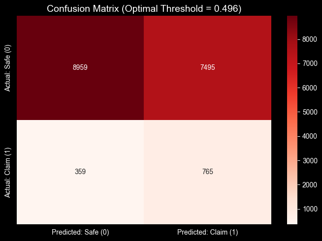
In imbalanced classification, the default 0.50 decision threshold is arbitrary. Because our models were trained with class_weight='balanced', the loss function was already reweighted to penalize missed positive claims, which brings the effective balance point near 0.50.

We now inspect the winning HistGradientBoosting model and tune the final operational decision boundary using Youden’s J statistic ($J = \text{TPR} - \text{FPR}$), finding the probability threshold that maximizes separation between True Positive Rate and False Positive Rate on unseen test data.

Code

from sklearn.metrics import (
    confusion_matrix,
    classification_report,
    roc_curve,
    roc_auc_score,
    average_precision_score
)

best_model = best_models[hist]

y_probs = best_model.predict_proba(X_test)[:, 1]
test_roc_auc = roc_auc_score(y_test, y_probs)
test_pr_auc = average_precision_score(y_test, y_probs)

fpr, tpr, thresholds = roc_curve(y_test, y_probs)
j_scores = tpr - fpr
best_index = np.argmax(j_scores)
optimal_threshold = thresholds[best_index]

print("=" * 50)
print("TEST SET GENERALIZATION:")
print(f"  -> ROC-AUC Score:          {test_roc_auc:.4f}")
print(f"  -> PR-AUC (Avg Precision): {test_pr_auc:.4f} (Baseline: {y_test.mean():.4f})")
print(f"DEFAULT THRESHOLD:           0.5000")
print(f"OPTIMAL THRESHOLD (Youden):  {optimal_threshold:.4f}")
print("=" * 50)

y_pred_optimal = (y_probs >= optimal_threshold).astype(int)

cm_optimal = confusion_matrix(y_test, y_pred_optimal)

plt.figure(figsize=(7, 5))
sns.heatmap(
    cm_optimal,
    annot=True,
    fmt='d',
    cmap='Reds',
    xticklabels=['Predicted: Safe (0)', 'Predicted: Claim (1)'],
    yticklabels=['Actual: Safe (0)', 'Actual: Claim (1)']
)
plt.title(f'Confusion Matrix (Optimal Threshold = {optimal_threshold:.3f})', fontsize=14)
plt.tight_layout()
plt.show()

print("\nClassification Report (Using Optimal Threshold):")
print(classification_report(y_test, y_pred_optimal))

==================================================
TEST SET GENERALIZATION:
  -> ROC-AUC Score:          0.6505
  -> PR-AUC (Avg Precision): 0.1061 (Baseline: 0.0639)
DEFAULT THRESHOLD:           0.5000
OPTIMAL THRESHOLD (Youden):  0.4956
==================================================


Classification Report (Using Optimal Threshold):
              precision    recall  f1-score   support

           0       0.96      0.54      0.70     16454
           1       0.09      0.68      0.16      1124

    accuracy                           0.55     17578
   macro avg       0.53      0.61      0.43     17578
weighted avg       0.91      0.55      0.66     17578

Precision (predicted claims that were claims divided by all predicted claims)

We achieved a precision of 9% (765 / (765 + 7495)).

While 9% might sound low at first glance, the baseline standard for a claim in this dataset is only 6%. This means if we pick any driver at random, there is only a 6% chance they will file a claim.

We isolated a risk pool where the chance of a claim is nearly double the average. The 7,495 drivers flagged by the model who didn’t crash yet are not necessarily safe drivers; they possess the exact same high-risk features as those who did crash. This risky behavior just hasn’t caught up to them yet.

Recall (predicted claims that were claims divided by all actual claims)

We achieved a recall of 68% (765 / (765 + 359)).

This means that out of the entire pool of drivers who actually got into an accident and filed a claim, the model identified and flagged 68% of them in advance.

Instead of being blindsided by these payouts, the business was warned about the majority of them ahead of time, allowing us to price their policies correctly.

Code

import numpy as np
import shap

print("Calculating SHAP values...")
explainer = shap.TreeExplainer(best_model)
shap_values = explainer.shap_values(X_test)
if isinstance(shap_values, list):
    shap_values_to_plot = shap_values[1]
elif len(shap_values.shape) == 3:
    shap_values_to_plot = shap_values[:, :, 1]
else:
    shap_values_to_plot = shap_values

plt.figure(figsize=(10, 6))
plt.title("SHAP Summary Plot: Drivers of Insurance Claims", fontsize=16, pad=20)
shap.summary_plot(shap_values_to_plot, X_test, plot_type="dot")

Calculating SHAP values...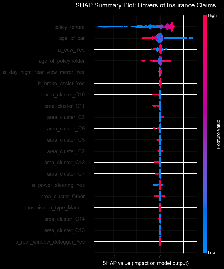

7. Conclusions

Brand new policyholders are the safest drivers, while longer policy tenure steadily increases claim risk.
The age of the vehicle acts as a massive risk shield. Brand new cars are most likely to file a claim, likely due to drivers using comprehensive coverage to fix minor damage on new investments.
Vehicles equipped with luxury features cluster together as a distinct risk factor, likely because their parts are significantly more expensive to repair, easily pushing minor incidents over the deductible.

Limitations

A cross-validated AUC of ~0.65 is typical for claim prediction — the signal in policy and vehicle attributes is genuinely weak, and results in this range are an honest ceiling rather than a modeling failure. Natural next steps: richer behavioral features (telematics — see the companion notebook), calibration analysis of the predicted probabilities, and a cost-based threshold instead of Youden’s J.

Predicting Car Insurance Claims

1. Data Audit

2. Data Engineering

The Plan

3. Multicollinearity and VIF

Why is it harmful?

Interpreting VIF Scores & Selecting the Threshold

The Iterative Pruning Rule

4. Statistical Modeling: Stepwise Logistic Regression

How Stepwise Selection Works

Why This Matters for Insurance

Key Insights from Feature Impacts (Log-Odds)

1. Vehicle Age is the Strongest Protective Factor (`age_of_car`: \(\beta = -3.53\), \(OR \approx 0.03\))

2. Policy Tenure Increases Claim Frequency (`policy_tenure`: \(\beta = +0.85\), \(OR \approx 2.33\))

3. Driver Demographics (`age_of_policyholder`: \(\beta = +0.31\), \(OR \approx 1.36\))

4. Geographic Territory Segmentation (`area_cluster`)

5. Safety Tech / Luxury Proxy (`is_brake_assist_Yes`: \(\beta = +0.09\), \(OR \approx 1.10\))

5. Model Bake-Off

6. Threshold Tuning

Precision (predicted claims that were claims divided by all predicted claims)

Recall (predicted claims that were claims divided by all actual claims)

7. Conclusions

Limitations

1. Data Audit

2. Data Engineering

The Plan

3. Multicollinearity and VIF

Why is it harmful?

Interpreting VIF Scores & Selecting the Threshold

The Iterative Pruning Rule

4. Statistical Modeling: Stepwise Logistic Regression

How Stepwise Selection Works

Why This Matters for Insurance

Key Insights from Feature Impacts (Log-Odds)

1. Vehicle Age is the Strongest Protective Factor (age_of_car: \(\beta = -3.53\), \(OR \approx 0.03\))

2. Policy Tenure Increases Claim Frequency (policy_tenure: \(\beta = +0.85\), \(OR \approx 2.33\))

3. Driver Demographics (age_of_policyholder: \(\beta = +0.31\), \(OR \approx 1.36\))

4. Geographic Territory Segmentation (area_cluster)

5. Safety Tech / Luxury Proxy (is_brake_assist_Yes: \(\beta = +0.09\), \(OR \approx 1.10\))

5. Model Bake-Off

6. Threshold Tuning

Precision (predicted claims that were claims divided by all predicted claims)

Recall (predicted claims that were claims divided by all actual claims)

7. Conclusions

Limitations

1. Vehicle Age is the Strongest Protective Factor (`age_of_car`: \(\beta = -3.53\), \(OR \approx 0.03\))

2. Policy Tenure Increases Claim Frequency (`policy_tenure`: \(\beta = +0.85\), \(OR \approx 2.33\))

3. Driver Demographics (`age_of_policyholder`: \(\beta = +0.31\), \(OR \approx 1.36\))

4. Geographic Territory Segmentation (`area_cluster`)

5. Safety Tech / Luxury Proxy (`is_brake_assist_Yes`: \(\beta = +0.09\), \(OR \approx 1.10\))