In this notebook, we will focus on predicting lung cancer risk based on patient data. Our approach includes: 1. Exploratory Data Analysis (EDA): Examining data distributions and correlations among features. 2. Feature Engineering & Selection: Handling multicollinearity using Variance Inflation Factor (VIF). 3. Supervised Modeling: Training Logistic Regression and Lasso models. 4. Model Evaluation & Interpretation: Comparing models using precision, recall, and F1-score, and explaining model predictions using SHAP values.
0. Data Loading
We load the lung cancer dataset (5,000 patients, 30 variables) together with its variable descriptions. The features span demographics (age, education_years), smoking behavior (smoking_years, cigarettes_per_day, pack_years), environmental exposures (air_pollution_index, radon_exposure), medical history (copd, family_history_cancer), and clinical measurements (oxygen_saturation, crp_level, xray_abnormal).
Note on the data: this is a synthetic educational dataset from Kaggle. Effect sizes are considerably stronger than in real clinical data, which is why the model separates classes more cleanly than any real-world screening tool would. The methodology is the point here, not the medical conclusions.
Code
import pandas as pddf_lung = pd.read_csv('data/lung_cancer.csv')print(df_lung.info())df_lung.describe()
import pandas as pddefinitions = pd.read_json('data/variables_descriptions.json')definitions.head()
name
description
0
age
Age of the individual in years
1
gender
Biological sex (0 = Female, 1 = Male)
2
education_years
Total years of formal education completed
3
income_level
Socioeconomic status on an ordinal scale (1 = ...
4
smoker
Indicates whether the individual has a history...
1. Data Preparation
First, we split our dataset into training and testing sets. We use a stratified split on the target variable lung_cancer_risk to ensure both sets have a representative proportion of the positive class.
Code
from sklearn.model_selection import train_test_splittarget_label ='lung_cancer_risk'y = df_lung[target_label].reset_index(drop=True)X = df_lung.drop(target_label, axis=1).reset_index(drop=True)
2. Exploratory Data Analysis (EDA)
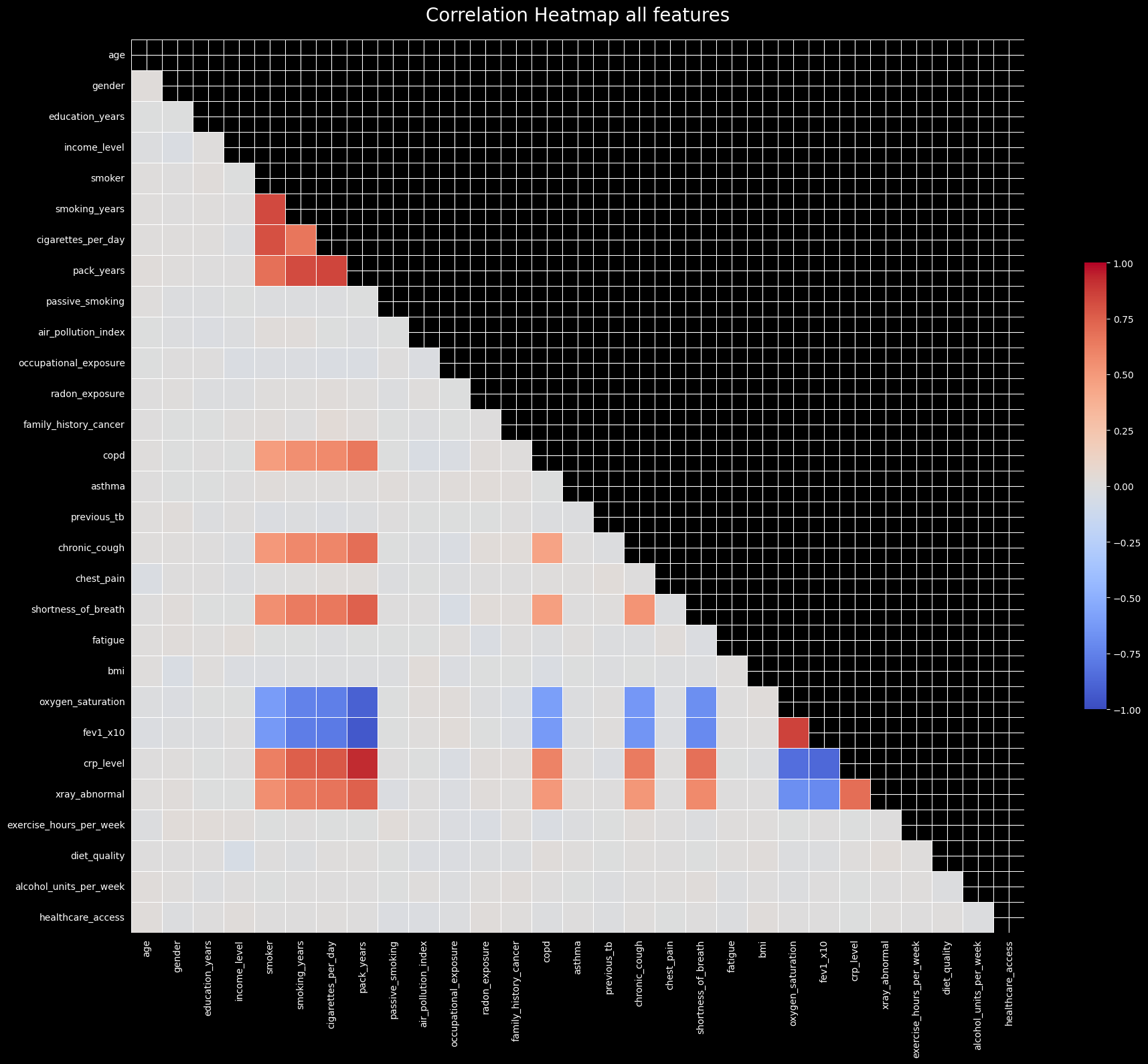
We visualize the correlations between all features. Highly correlated features can introduce multicollinearity, which might destabilize linear models like Logistic Regression.
Code
from statsmodels_utils import plot_correlation_heatmapplot_correlation_heatmap(X, 'Correlation Heatmap all features')
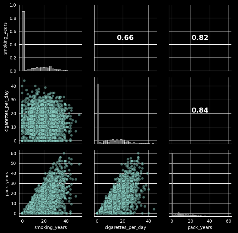
Let’s take a closer look at the relationships between smoking-related variables, as they are typically highly correlated.
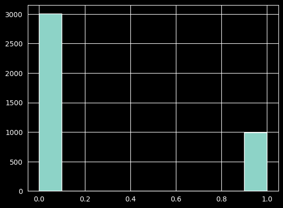
We hold out 20% of the data for testing, stratifying on the target so both splits keep the same class mix. The histogram below confirms the class imbalance: roughly 3 in 4 patients are negative. This matters later — it is why we look beyond accuracy when evaluating, and why the regularized benchmark uses class weighting.
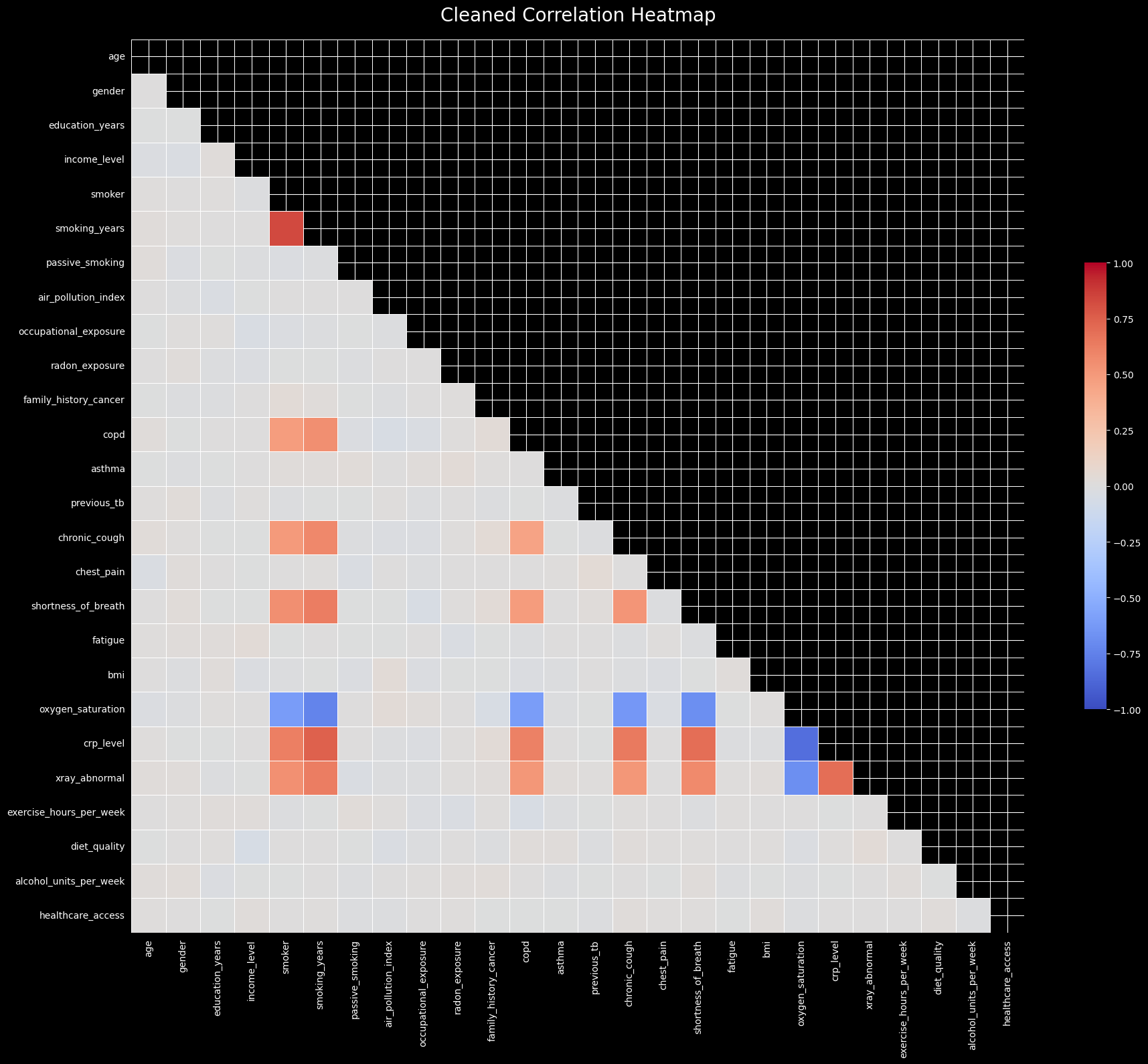
As seen in the correlation heatmap and pair plot, there are strong correlations among certain features (like pack_years and smoking_years). This indicates a potential multicollinearity issue, which we can quantify using the Variance Inflation Factor (VIF). We will recursively calculate VIF and drop features that exceed a threshold to ensure model stability.
Starting VIF Multicollinearity Check...

----------------------------------------

[DROPPED] 'pack_years'
  * VIF Score: 35.66 (Overlap: 97.2%)
  * Primary Suspects (Highest pairwise correlations with this feature):
      - fev1_x10 (0.95)
      - crp_level (0.92)
      - oxygen_saturation (0.91)
  * Current Runner-Ups (Watch these scores drop in the next loop!):
      - cigarettes_per_day: 14.60
      - smoking_years: 13.52
      - smoker: 12.77
------------------------------

[DROPPED] 'cigarettes_per_day'
  * VIF Score: 10.40 (Overlap: 90.4%)
  * Primary Suspects (Highest pairwise correlations with this feature):
      - smoker (0.81)
      - fev1_x10 (0.79)
      - crp_level (0.79)
  * Current Runner-Ups (Watch these scores drop in the next loop!):
      - smoker: 10.22
      - smoking_years: 9.84
      - fev1_x10: 7.19
------------------------------

[DROPPED] 'fev1_x10'
  * VIF Score: 6.33 (Overlap: 84.2%)
  * Primary Suspects (Highest pairwise correlations with this feature):
      - crp_level (0.88)
      - oxygen_saturation (0.86)
      - smoking_years (0.77)
  * Current Runner-Ups (Watch these scores drop in the next loop!):
      - crp_level: 5.36
      - smoking_years: 5.03
      - oxygen_saturation: 4.73
------------------------------
----------------------------------------
VIF Check Complete!
Features dropped: 3
4. Modeling: Logistic Regression
We train a Logistic Regression model (statsmodels Logit) and select features via backward elimination: starting from the full cleaned feature set, we iteratively drop the least significant feature (highest p-value above 0.05) and refit, until every remaining coefficient is statistically significant. This yields a compact, interpretable model where every retained feature earns its place.
Code
# go for stats model logitfrom statsmodels_utils import stepwise_selection, backward_eliminationimport statsmodels.api as smlogit_model = sm.Logitfinal_model_logit, features = backward_elimination(logit_model, X_train_clean, y_train, disp=False, warn_convergence=False)print(f"Optimal features: {features}")final_model_logit.summary()
Possibly complete quasi-separation: A fraction 0.67 of observations can be perfectly predicted. This might indicate that there is complete quasi-separation. In this case some parameters will not be identified.
5. Model Evaluation
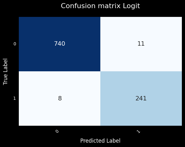
We evaluate on the held-out test set using a 0.5 probability threshold. Accuracy alone is misleading here — only ~25% of cases are positive, so a model that always predicts “no cancer” would score ~75% while being clinically useless.
The metric that matters most in this context is Recall (sensitivity): of the patients who actually have cancer, how many did we catch? In a screening setting, a false negative (a missed cancer) is far more costly than a false positive (an unnecessary follow-up test).
As a robustness check we fit a second logistic regression, this time with an L1 (lasso) penalty via scikit-learn. Instead of dropping features by p-value, the L1 penalty performs feature selection implicitly by shrinking weak coefficients to exactly zero. class_weight='balanced' compensates for the class imbalance seen above.
Code
from sklearn.linear_model import LogisticRegression# L1-regularized *logistic* regression (a true apples-to-apples comparison# with the statsmodels Logit above; sklearn's Lasso is linear regression).clf = LogisticRegression(penalty='l1', solver='liblinear', C=1.0, class_weight='balanced', random_state=seed)clf.fit(X_train, y_train)clf_selected_features = X_train.columns[clf.coef_[0] !=0]y_pred_lasso = clf.predict(X_test[X_train.columns])print("Lasso selected features: ", clf_selected_features.tolist())print("Stepwise selected features: ", features)print("Common features: ", [features[i] for i inrange(len(features)) if features[i] in clf_selected_features])print("Logit Excluded features from Lasso: ", clf_selected_features.difference(features).tolist())print("Lasso Excluded features from Logit: ", list(set(features).difference(clf_selected_features)))
Both approaches perform feature selection, but by different mechanisms: the L1 penalty shrinks uninformative coefficients exactly to zero during optimization, while backward elimination drops features by statistical significance. Comparing the two selected feature sets is a useful robustness check — features chosen by both methods are the ones to trust most.
When comparing the two models, we weigh Recall above raw accuracy for the clinical reasons outlined above. The backward-elimination Logit remains our deployment choice: its coefficients map one-to-one to interpretable log-odds contributions per feature, its feature set was vetted for multicollinearity beforehand (VIF), and its statistical summary (p-values, confidence intervals) supports the kind of scrutiny expected in a biostatistics setting.
The regularized model serves as a sanity check that a different selection mechanism lands on a similar signal — not as a competing deployment candidate.
6. Saving Model Artifacts
We will serialize and save the coefficients of our chosen Logistic Regression model, along with the list of selected features. This will allow us to reproduce the scoring and deploy the model for future predictions.
Code
# we save the coefficients for further predictionsimport jsonimport osout_dir ='../frontend/public'logit_filename ='logit_weights'coeffs = final_model_logit.params.tolist()os.makedirs(out_dir, exist_ok=True)withopen(f"{out_dir}/{logit_filename}.json", 'w') as f: json.dump(coeffs, f, indent=4)print(f"Model coefficients saved to '{out_dir}/{logit_filename}.json'") features_filename =f"{logit_filename}_features.json"# we save the features and their order for referencewithopen(f"{out_dir}/{features_filename}", 'w') as f:# the add the const as the first feature json.dump(['const',*features], f, indent=4)print(f"Features saved to '{out_dir}/{logit_filename}_features.json'")
7. Model Interpretability with SHAP
To understand how our Logistic Regression model makes its predictions, we will analyze the impact of individual features using SHAP (SHapley Additive exPlanations). This allows for both global and local interpretability.
Code
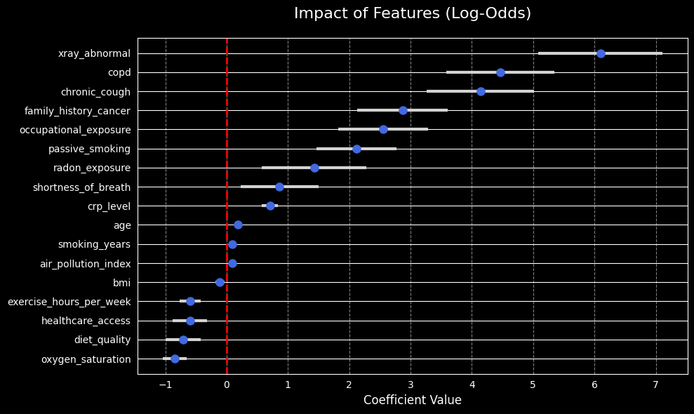
from statsmodels_utils import plot_coeffeatures_impact_image =f'{plot_folder}/features_impact.jpg'plot_coef(final_model_logit, plot_file=features_impact_image)
Plot saved successfully to: ../frontend/public/plots/features_impact.jpg
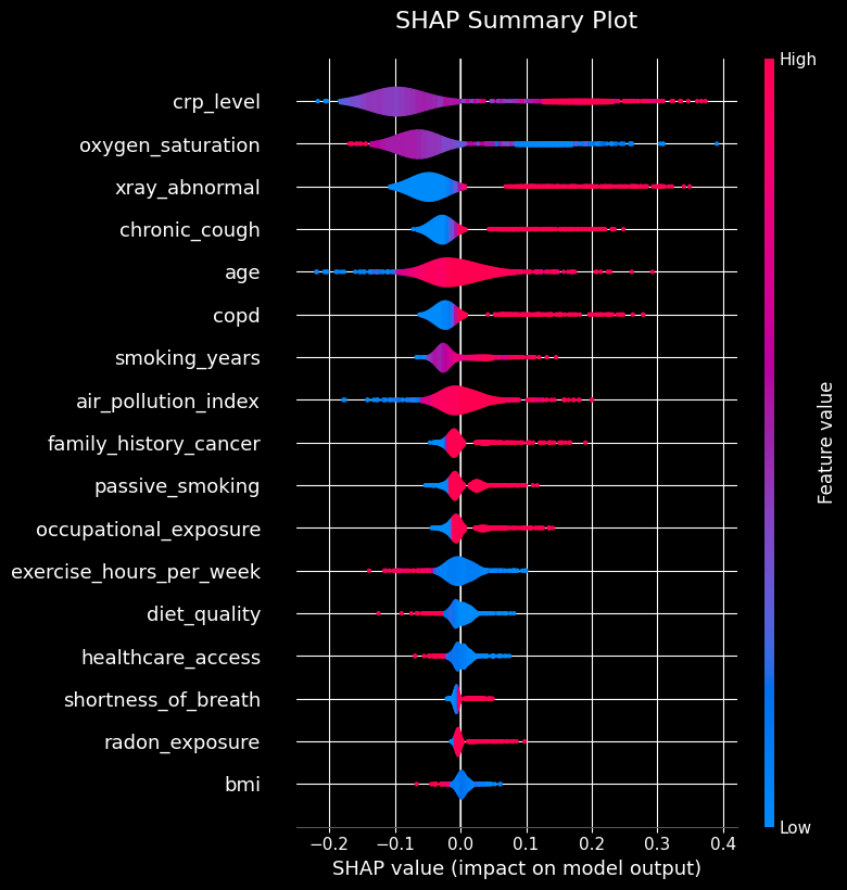
Global Explanations: SHAP Summary
The SHAP summary plot gives us a bird’s-eye view of feature importance and the direction of the relationship between feature values and the prediction.
Plot saved successfully to: ../frontend/public/plots/shap_summary.jpg
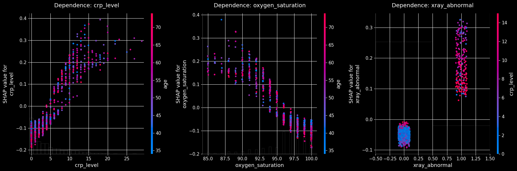
As seen in the plots above, the top three most influential features (crp_level, oxygen_saturation, and xray_abnormal) are all derived from clinical laboratory tests and imaging. This reinforces the clinical validity of the model, as these objective medical measurements strongly drive the predictions.
The SHAP bar plot aggregates the mean absolute SHAP values, providing a clear ranking of overall feature importance across the entire dataset.
Code
from statsmodels_utils import plot_shap_barshap_feature_importance_image =f'{plot_folder}/shap_feature_importance.jpg'plot_shap_bar(final_model_logit, with_constant, plot_file=shap_feature_importance_image)
Plot saved successfully to: ../frontend/public/plots/shap_feature_importance.jpg
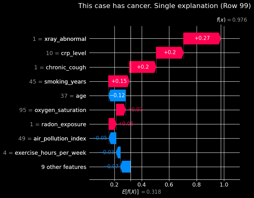
Local Explanations: Single Prediction
We can also use SHAP to explain individual predictions. Let’s look at a specific patient (e.g., index 99) to see how their specific feature values pushed the model’s prediction probability above or below the base value.
Code
from statsmodels_utils import plot_shap_waterfall_singleindex_to_plot =99predicted_probability = final_model_logit.predict(with_constant.iloc[[index_to_plot]])label =f"This case {"has"if predicted_probability.iloc[0] >0.5else"does not have"} cancer."single_explanation_image =f'{plot_folder}/single_explanation.jpg'plot_shap_waterfall_single( final_model_logit, with_constant, row_index=index_to_plot, title=f"{label} Single explanation", plot_file=single_explanation_image)
Plot saved successfully to: ../frontend/public/plots/single_explanation.jpg
For the patient at index 99, we can see exactly how the model arrived at its positive prediction. Notably, having an abnormal X-ray (xray_abnormal = 1) is a primary driver, increasing the log-odds of the prediction. Other clinical features and medical history also significantly push the risk higher.
Feature Dependence
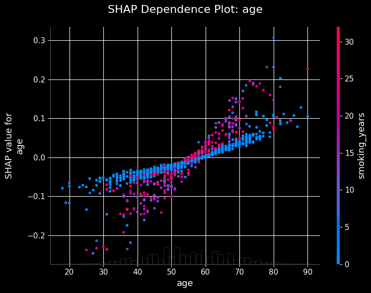
SHAP dependence plots show the marginal effect of a feature on the prediction. Let’s visualize how the model’s output depends on specific variables like age.
Code
from statsmodels_utils import plot_shap_dependenceshap_dependence_image =f'{plot_folder}/shap_dependence.jpg'plot_shap_dependence(final_model_logit, with_constant, 'age', plot_file=shap_dependence_image)
Plot saved successfully to: ../frontend/public/plots/shap_feature_importance.jpg
Code
from statsmodels_utils import plot_top_shap_dependenceplot_shap_dependence_image =f'{plot_folder}/shap_dependence_top.jpg'plot_top_shap_dependence(final_model_logit, with_constant, top_n=3, plot_file=plot_shap_dependence_image)
What we built. An end-to-end, interpretable classifier for lung cancer risk: multicollinearity pruning (VIF) → backward-elimination Logit → benchmark against an L1-regularized logistic regression → SHAP interpretability → coefficient export for in-browser inference.
Key findings.
Clinical measurements dominate. The three most influential features — crp_level, oxygen_saturation, and xray_abnormal — are all objective lab/imaging results rather than self-reported behaviors. That pattern is what you would hope a credible medical model learns.
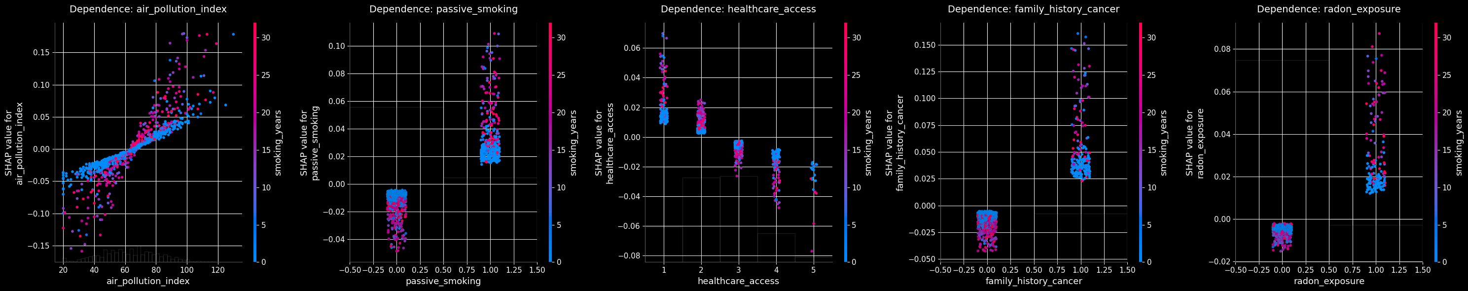
Behavioral and environmental factors contribute coherent second-order signal. Smoking history, passive smoking, radon and occupational exposures all push risk in the medically expected direction (as seen in the SHAP summary and dependence plots).
Feature selection was robust. Multicollinear duplicates (e.g. pack_years vs smoking_years) were removed by VIF before fitting, and the surviving feature set is statistically significant end to end.
Interpretability comes free. Because the deployed model is a plain Logit, the browser app reproduces its exact probabilities with a dot product and a sigmoid — no server, no approximation, and every slider’s effect on the score is directly traceable to a coefficient.
Limitations & future work.
The dataset is synthetic; coefficients (some odds ratios are implausibly large) and metrics should not be read as clinical findings.
Single train/test split — cross-validated metrics with confidence intervals would harden the evaluation.
The 0.5 decision threshold is arbitrary for a screening context; threshold tuning against a recall target (or a cost-sensitive analysis) is the natural next step.
No probability calibration check yet (reliability curve / Brier score) — worth adding since the app surfaces raw probabilities to users.