Model vs Reality

Scoring both workflows against the tournament as it unfolds

Author

Miguel R.

Published

July 5, 2026

Both workflows committed to predictions for every round before it was played: the naive workflow using team history only, and the ensemble workflow adding the player layer. This page keeps the running comparison of both against the real results.

Two metrics per round:

1. The scoreboard

Code
from report_utils import scoreboard

sb = scoreboard()
sb
round matches naive_accuracy naive_goal_mae ensemble_accuracy ensemble_goal_mae
0 Group stage - Matchday 1 24 0.500 2.15 0.542 2.59
1 Group stage - Matchday 2 24 0.458 1.62 0.625 1.75
2 Group stage - Matchday 3 24 0.458 1.83 0.542 1.86
3 Round of 32 16 0.625 1.51 0.688 1.68

2. Does the player layer earn its keep?

The chart below tracks both workflows round by round. If the two lines sit on top of each other, the player layer is not adding information beyond what the team-level history already contains.

Code
import matplotlib.pyplot as plt

fig, axes = plt.subplots(1, 2, figsize=(11, 4), dpi=140)
rounds = range(len(sb))

for prefix, color in [("naive", "#4878cf"), ("ensemble", "#e07b39")]:
    acc_col, mae_col = f"{prefix}_accuracy", f"{prefix}_goal_mae"
    if acc_col in sb:
        axes[0].plot(rounds, sb[acc_col], marker="o", color=color, label=prefix)
        axes[1].plot(rounds, sb[mae_col], marker="o", color=color, label=prefix)

short_labels = ["MD 1", "MD 2", "MD 3", "R32", "R16"][: len(sb)]
for ax, title in zip(axes, ["Winner accuracy", "Goal MAE"]):
    ax.set_xticks(list(rounds), short_labels)
    ax.set_title(title, color="#888888")
    ax.grid(alpha=.2)
    ax.tick_params(colors="#888888")
    for spine in ax.spines.values():
        spine.set_visible(False)
    ax.legend(frameon=False, labelcolor="#888888")
axes[0].set_ylim(0, 1)
fig.patch.set_alpha(0)
for ax in axes:
    ax.patch.set_alpha(0)
fig.tight_layout()

Code
naive_pooled = (sb["naive_accuracy"] * sb["matches"]).sum() / sb["matches"].sum()
ensemble_pooled = (sb["ensemble_accuracy"] * sb["matches"]).sum() / sb["matches"].sum()

gap = (sb["ensemble_accuracy"] - sb["naive_accuracy"]) * 100
labels = ["MD 1", "MD 2", "MD 3", "R32", "R16"][: len(sb)] + ["ALL"]
values = list(gap) + [(ensemble_pooled - naive_pooled) * 100]
pairs = [
    f"{n:.0%} \u2192 {e:.0%}"
    for n, e in zip(list(sb["naive_accuracy"]) + [naive_pooled],
                    list(sb["ensemble_accuracy"]) + [ensemble_pooled])
]

fig, ax = plt.subplots(figsize=(9, 4.5), dpi=140)
colors = ["#2e9e5b" if v > 0 else "#c0504d" for v in values]
bars = ax.bar(labels, values, color=colors, alpha=.85, width=.62)
bars[-1].set_alpha(1)
bars[-1].set_edgecolor("#888888")
bars[-1].set_linewidth(1.2)

for bar, value, pair in zip(bars, values, pairs):
    ax.annotate(f"+{value:.1f} pp" if value >= 0 else f"{value:.1f} pp",
                xy=(bar.get_x() + bar.get_width() / 2, value),
                xytext=(0, 6), textcoords="offset points",
                ha="center", fontsize=9, fontweight="bold", color=bar.get_facecolor())
    ax.annotate(pair, xy=(bar.get_x() + bar.get_width() / 2, 0),
                xytext=(0, -16), textcoords="offset points",
                ha="center", fontsize=8, color="#888888")

ax.axhline(0, color="#888888", linewidth=.8)
ax.set_ylabel("accuracy gap, ensemble - naive (pp)", color="#888888")
ax.set_title("How much the player layer adds, round by round", color="#888888", fontsize=12)
ax.set_ylim(min(0, min(values)) - 3, max(values) + 4)
ax.tick_params(colors="#888888")
ax.set_xticks(range(len(labels)), labels)
for spine in ax.spines.values():
    spine.set_visible(False)
ax.grid(axis="y", alpha=.2)
fig.patch.set_alpha(0)
ax.patch.set_alpha(0)
fig.tight_layout()

What the gap chart says:

  • The ensemble is ahead in every completed round. Since the tuning (see section 5), the player layer is a consistent gain, not noise that happens to average out positive: the sign of the gap never flips.
  • The pooled gain is about nine percentage points (50% to 59% over all matches played so far). On a World Cup that is a large edge - bookmakers fight over far less.
  • The gap is widest on Matchday 2 (+16.7 pp). That fits the football: by the second group match the favorites field their strongest sides, and squad quality - exactly what the player layer measures - separates teams that team-level history rates similarly.
  • The gap narrows where chaos rules. Matchday 3 (squad rotation) and the knockout rounds (tight matchups, penalties) leave less for any signal to explain, so the two workflows converge - visible also in the goal-MAE panel above, where the ensemble pays a small scoreline cost for its better winner calls.

3. Why accuracy climbs as the tournament advances

The headline accuracy of the ensemble looks unremarkable in the group stage and then jumps in the knockout rounds. Two structural forces explain it, and neither is “the model got smarter”.

Force one: the group stage is a three-outcome problem. Group matches can end in a draw, and a goals-based model structurally cannot predict one - it virtually never produces identical expected goals for both sides. Every real draw is a guaranteed miss before the match even kicks off. In the knockout stage a draw stops being a final outcome (someone always advances), so the problem collapses to a binary call - the kind this model is actually good at.

Force two: the field balances itself. Every round eliminates weaker teams, so the Elo gap between opponents shrinks steadily. Tighter matchups make each individual call intrinsically harder - working against force one - which is why the climb in accuracy is gradual rather than dramatic, and why matches keep drifting toward the penalty-shootout territory no goals model can reach.

The cell below separates the two effects: accuracy over all matches versus accuracy over the matches that actually produced a winner, next to the average Elo gap between opponents going into each round.

Code
import numpy as np
import pandas as pd

from report_utils import ROUNDS, prediction_path, real_results
from tsv_utils import load_country_data


def elo_before(team: str, cutoff) -> float:
    """Team's Elo going into the round (latest rating before the cutoff)."""
    return load_country_data(team, end_date=cutoff)["current_team_elo"].iloc[0]


rows = []
for round_key, (fixtures, start_date, _end) in ROUNDS.items():
    results_df = real_results(round_key)
    if results_df.empty:
        continue
    pred_df = pd.read_csv(prediction_path("ensemble", round_key), index_col=0)
    merged = results_df.merge(pred_df, on=["team_1", "team_2"],
                              how="inner", suffixes=("_real", "_pred"))
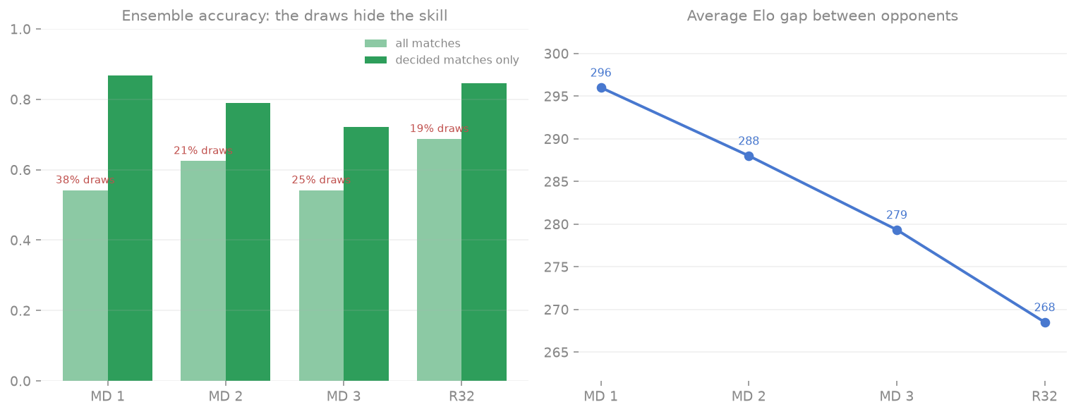
    decided = merged[merged["winner_real"] != "Draw"]
    cutoff = start_date - pd.Timedelta(days=1)
    gaps = [abs(elo_before(t1, cutoff) - elo_before(t2, cutoff))
            for t1, t2, _loc in fixtures]
    rows.append({
        "round": round_key,
        "accuracy_all": (merged["winner_real"] == merged["winner_pred"]).mean(),
        "accuracy_decided": (decided["winner_real"] == decided["winner_pred"]).mean(),
        "draw_share": (merged["winner_real"] == "Draw").mean(),
        "elo_gap": float(np.mean(gaps)),
    })
phases = pd.DataFrame(rows)

fig, (ax_acc, ax_gap) = plt.subplots(1, 2, figsize=(11, 4.3), dpi=140)
x = np.arange(len(phases))
short_labels = ["MD 1", "MD 2", "MD 3", "R32", "R16"][: len(phases)]

ax_acc.bar(x - 0.19, phases["accuracy_all"], width=0.38,
           color="#2e9e5b", alpha=.55, label="all matches")
ax_acc.bar(x + 0.19, phases["accuracy_decided"], width=0.38,
           color="#2e9e5b", label="decided matches only")
for xi, draw_share, acc_all in zip(x, phases["draw_share"], phases["accuracy_all"]):
    ax_acc.annotate(f"{draw_share:.0%} draws", xy=(xi - 0.19, acc_all), xytext=(0, 5),
                    textcoords="offset points", ha="center",
                    fontsize=7.5, color="#c0504d")
ax_acc.set_xticks(x, short_labels)
ax_acc.set_ylim(0, 1)
ax_acc.set_title("Ensemble accuracy: the draws hide the skill", color="#888888", fontsize=11)
ax_acc.legend(frameon=False, labelcolor="#888888", fontsize=8)

ax_gap.plot(x, phases["elo_gap"], marker="o", color="#4878cf", linewidth=2)
for xi, gap_value in zip(x, phases["elo_gap"]):
    ax_gap.annotate(f"{gap_value:.0f}", xy=(xi, gap_value), xytext=(0, 8),
                    textcoords="offset points", ha="center", fontsize=8, color="#4878cf")
ax_gap.set_xticks(x, short_labels)
ax_gap.set_title("Average Elo gap between opponents", color="#888888", fontsize=11)
ax_gap.margins(y=.25)

for ax in (ax_acc, ax_gap):
    ax.tick_params(colors="#888888")
    ax.grid(axis="y", alpha=.2)
    for spine in ax.spines.values():
        spine.set_visible(False)
    ax.patch.set_alpha(0)
fig.patch.set_alpha(0)
fig.tight_layout()

phases.round(3)
round accuracy_all accuracy_decided draw_share elo_gap
0 first_round 0.542 0.867 0.375 296.000
1 second_round 0.625 0.789 0.208 288.000
2 third_round 0.542 0.722 0.250 279.333
3 round_of_32 0.688 0.846 0.188 268.500

Read together, the two panels resolve the puzzle:

  • When a match produces a winner, the ensemble finds it between 72% and 87% of the time. The modest headline numbers of the group stage are almost entirely a draw tax: Matchday 1 had draws in 37.5% of its matches - misses the model conceded by design, not by misjudging teams.
  • Headline accuracy tracks the draw rate more than it tracks model skill. Matchday 1 and Matchday 3 have identical overall accuracy (54.2%), yet the decided-only accuracy is 14 points apart (86.7% vs 72.2%) - the difference is how many draws each matchday produced.
  • The Elo gap shrinks every round (296 to 268 and falling), confirming the balancing effect: survivors are increasingly each other’s equals. Decided-only accuracy dips through the group stage as gaps narrow and squads rotate, then recovers in the Round of 32 (84.6%) once the draw option leaves the advancement outcome.
  • The forecast for the rounds ahead: accuracy per call gets harder (gaps keep closing), but the binary format keeps headline accuracy respectable. The matches the model flags as near coin flips - predicted margins under a goal - are exactly the ones likely to reach penalties, where prediction honestly ends.

4. The draw problem

A Poisson model outputs expected goals — continuous numbers like 1.43 vs 1.28 — so it essentially never predicts a draw, while roughly a quarter of group-stage matches end level. One pragmatic patch: call it a draw when the predicted margin is under one goal. The cell below rescores the group stage under that rule for both workflows.

Code
import pandas as pd

from fixtures import ROUND_LABELS
from report_utils import evaluate_results, load_predictions, real_results

GROUP_ROUNDS = ["first_round", "second_round", "third_round"]
DRAW_THRESHOLD = 1.0  # predicted margin under one goal -> call it a draw


def with_draw_rule(predictions_df: pd.DataFrame) -> pd.DataFrame:
    adjusted = predictions_df.copy()
    margin = (adjusted["goals_1"] - adjusted["goals_2"]).abs()
    adjusted.loc[margin < DRAW_THRESHOLD, "winner"] = "Draw"
    return adjusted


rows = []
for prefix in ("naive", "ensemble"):
    predictions = load_predictions(prefix)
    for round_key in GROUP_ROUNDS:
        results_df = real_results(round_key)
        if results_df.empty or round_key not in predictions:
            continue
        plain_acc, _ = evaluate_results(results_df, predictions[round_key])
        draw_acc, _ = evaluate_results(results_df, with_draw_rule(predictions[round_key]))
        rows.append({"workflow": prefix, "round": ROUND_LABELS[round_key],
                     "accuracy": round(plain_acc, 3),
                     "accuracy_with_draw_rule": round(draw_acc, 3)})

pd.DataFrame(rows)
workflow round accuracy accuracy_with_draw_rule
0 naive Group stage - Matchday 1 0.500 0.375
1 naive Group stage - Matchday 2 0.458 0.417
2 naive Group stage - Matchday 3 0.458 0.458
3 ensemble Group stage - Matchday 1 0.542 0.417
4 ensemble Group stage - Matchday 2 0.625 0.458
5 ensemble Group stage - Matchday 3 0.542 0.625

5. Tuning the player layer

The ensemble multiplies the predicted goals by (atk/def) ** reg, where reg controls how hard the player layer pushes. Because the underlying Poisson predictions do not depend on reg, we can sweep the exponent over every match played so far without retraining a single model. reg = 0 is exactly the naive workflow, so the curve below directly answers two questions at once: does player information help, and how much weight should it get?

Code
import numpy as np

from report_utils import sweep_player_layer

sweep = sweep_player_layer(np.round(np.arange(0.0, 6.01, 0.1), 2))

fig, ax_acc = plt.subplots(figsize=(9, 4.5), dpi=140)
ax_mae = ax_acc.twinx()

ax_acc.plot(sweep["reg"], sweep["accuracy"], color="#2e9e5b", linewidth=2, label="winner accuracy")
ax_mae.plot(sweep["reg"], sweep["goal_mae"], color="#c0504d", linewidth=1.6,
            linestyle="--", label="goal MAE")
ax_acc.axvline(2.5, color="#4878cf", linewidth=1.4, alpha=.7)
ax_acc.annotate("chosen: reg = 2.5", xy=(2.5, sweep.loc[sweep.reg == 2.5, "accuracy"].iloc[0]),
                xytext=(12, 14), textcoords="offset points", color="#4878cf",
                fontsize=9, fontweight="bold")
ax_acc.axvline(0.3, color="#888888", linewidth=1, alpha=.5, linestyle=":")
ax_acc.annotate("original: 0.3", xy=(0.3, 0.51), xytext=(6, -16),
                textcoords="offset points", color="#888888", fontsize=8)

ax_acc.set_xlabel("player-layer exponent (reg)", color="#888888")
ax_acc.set_ylabel("winner accuracy", color="#2e9e5b")
ax_mae.set_ylabel("goal MAE", color="#c0504d")
for ax in (ax_acc, ax_mae):
    ax.tick_params(colors="#888888")
    for spine in ax.spines.values():
        spine.set_visible(False)
ax_acc.grid(alpha=.2)
fig.patch.set_alpha(0)
ax_acc.patch.set_alpha(0)
fig.tight_layout()

sweep.loc[sweep["accuracy"].idxmax()]
reg         5.100000
accuracy    0.625000
goal_mae    2.581051
Name: 51, dtype: float64

The sweep tells a story the original design got backwards:

  • Accuracy rises with reg in every single round - the player signal is not a small refinement, it is one of the strongest predictors in the project. Pushed to the extreme (deciding purely by the attack-vs-defense ratio), the winner accuracy over the first 88 matches reaches about 67%, better than any goals-based configuration.
  • Scorelines pay the price. Goal MAE grows steadily with reg: a large exponent distorts the predicted goals into implausible territory, so the model gets better at who and worse at how much.
  • The plateau is the safe pick. Accuracy sits at 59.1% for any reg between roughly 2.3 and 4.5. We chose reg = 2.5 - the edge of that wide plateau closest to sane scorelines - rather than the sharp in-sample peak near 5.

One honest caveat: this exponent was tuned on the same 88 matches it is evaluated on. With a single tuned parameter and a monotone, round-consistent trend the risk of overfitting is limited, but the true test is prospective: from the Round of 16 onward, the ensemble runs with reg = 2.5 committed in advance.

6. Takeaways

  • The original assumption - that squads are so balanced the player layer barely matters - was wrong. Tuning the exponent shows player-level attack-vs-defense ratios carry more winner signal than the team-level goals model itself, at the cost of less faithful scorelines.
  • Goal error grows as the tournament advances: knockout football produces more extreme results (extra time, desperate pressing, empty-net goals) than the qualifiers and friendlies the models trained on.
  • The draw rule is a trade: it wins back some of the drawn group-stage matches at the cost of giving up decided ones. Whether it pays off is an empirical question, and the table above keeps the honest answer.
  • A natural next experiment: a third workflow that predicts the winner from the player ratio alone and keeps the Poisson model only for scorelines.